Download
1 / 75
1.01k likes | 2.17k Vues
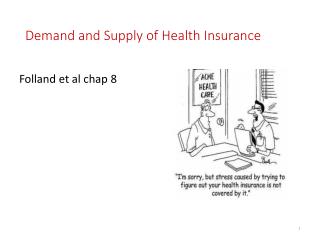
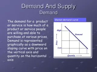
Demand and Supply of Health Insurance. Bhattacharya et al chap 7 and 11. Why buy insurance?. Demand for insurance driven by the fear of the unknown -Hedge against risk and the possibility of bad outcomes Purchasing insurance means forfeiting income in good times to get money in bad times

E N D
Demand and Supply of Health Insurance. Bhattacharya et al chap 7 and 11
Why buy insurance? • Demand for insurance driven by the fear of the unknown -Hedge against risk and the possibility of bad outcomes • Purchasing insurance means forfeiting income in good times to get money in bad times • If bad times avoided, then money lost • Ex: The individual who buys health insurance but never visits the hospital might have been better off spending that income elsewhere.
Risk aversion • Hence, risk aversion drives demand for insurance • We can model risk aversion through utility from income U(I) • Utility increases with income: U(I) > 0 • Marginal utility for income is declining: U(I) < 0
Income and utility • Graphically, • Utility increasing with income U’(I) > 0 • Marginal utility decreasing U’’(I) > 0
Adding uncertainty to the model • An individual does not know whether she will become sick, but she knows the probability of sickness is pbetween 0 and 1 • Probability of sickness is p • Probability of staying healthy is (1 – p) • If she gets sick, medical bills and missed work will reduce her income • IS = income if she does get sick • IH > IS = income if she remains healthy
Expected value • The expected value of a random variable X, E[X], is the sum of all the possible outcomes of X weighted by each outcome’s probability • If the outcomes are x1, x2, . . . , xn, and the probabilities for each outcome are p1, p2, . . . , pn respectively, then: E[X] = p1 x1 + p2 x2 + · · · + pnxn • In our individual’s case, the formula for expected value of income E[I]: E[I] = p IS + (1- p) IH
Example: expected value • Suppose we offer a starving graduate student a choice between two possible options, a lottery and a certain payout: A: a lottery that awards $500 with probability 0.5 and $0 with probability 0.5. B: a check for $250 with probability 1. • The expected value of both the lottery and the certain payout is $250: E[I] = p IS + (1- p) IH E[A] = .5(500) + .5(0) = $250 E[B] = 1(250) = $250
People prefer certain outcomes • Studies find that most people prefer certain payouts over uncertain scenarios • If a student says he prefers uncertain option, what does that imply about his utility function? • To answer this question, we need to define expected utility for a lottery or uncertain outcome.
Expected Utility • The expected utility from a random payout X E[U(X)] is the sum of the utility from each of the possible outcomes, weighted by each outcome’s probability. • If the outcomes are x1, x2, . . . , xn, and the probabilities for each outcome are p1, p2, . . . , pn respectively, then: E[U(X)] = p1 U(x1) + p2 U(x2) + · · · + pn U(xn)
Example • The student’s preference for option B over option A implies that his expected utility from B, is greater than his expected utility from A: E[U(B)] ≥ E[U(A)] U($250) ≥ 0.5 U($500) + 0.5 U($0) • In this case, even though the expected values of both options are equal, the student prefers the certain payout over the less certain one. • This student is acting in a risk-averse manner over the choices available.
Expected utility without insurance • Lottery scenario similar to case of insurance customer • She gains a high income IH if healthy, and low income IS if sick. • Uncertainty about which outcome will happen, though she knows the probability of becoming sick is p • Expected utility E[U(I)] is: E[U(I)] = p U(IS) + (1- p) U(IH)
E[U(I)] and probability of sickness • Consider a case where the person is sick with certainty (p = 1): • E[U] = U(IS) equals the utility from certain income IS (Point S) • Consider case where person has no chance of becoming sick (p = 0): • E[U] = U(IH) equals utility from certain income IH (Point H)
What if p lies between 0 and 1? For p between 0 and 1, expected utility falls on a line segment between S and H
Ex: p = 0.25 • For p = 0.25, person’s expected income is: E[I] = 0.25·IS + (1 - .25)·IH • Utility at that expected income is E[U(I)] (Point A)
Expected utility and expected income • Crucial distinction between • Expected utility E[U(I)] • Utility from expected income U(E[I]) • For risk-averse people, U(E[I]) > E[U(I)]
Risk-averse individuals Synonymous definitions of risk-aversion: • Prefer certain outcomes to uncertain ones with the same expected income. • Prefers the utility from expected income to the expected utility from uncertain income • U(E[I]) > E[U(I)] • Concave utility function • U’(I) > 0 • U’’(I) < 0
A basic health insurance contract • Customer pays an upfront fee • Payment ris known as the insurance premium • If ill, customer receives q-- the insurance payout • If healthy, customer receives nothing • Either way, customer loses the upfront fee • Customer’s final income is: • Sick: IS + q – r • Healthy: IH + 0 – r
Income with insurance • Let IH’ and IS’ be income with insurance • Sick: IS’ = IS + q – r • Healthy: IH’ = IH + 0 – r • Remember that risk-averse consumers want to avoid uncertainty • For them, optimally IH’ = IS’
Full insurance • Full insurance means no income uncertainty IS’ = IH’ • Final income is state-independent • Regardless of healthy or sick, final income is the same • Risk-averse individuals prefer full insurance to partial insurance (given the same price)
Full insurance payout • State independence implies • IH’ = IS’ • So IH + 0 – r = IS + q – r IH = IS + q q = IH – IS • The payout from a full insurance contract is difference between incomes without insurance
Actuarially fair insurance • Actuarially fair means that insurance is a fair bet • i.e. the premium equals the expected payout r = p q • Insurer makes zero profit/loss from actuarially fair insurance in expectation
Actuarially fair, full insurance Notice consumers with actuarially fair, full insurance achieve their expected income with certainty!
Insurance and risk aversion • As we have seen, simply by reducing uncertainty, insurance can make this risk-averse individual better off. • Relative to the state of no insurance, with insurance she loses income in the healthy state (IH > IH) and gains income in the sick state (IS < IS). • In other words, the risk-averse individual willingly sacrifices some good times in the healthy state to ease the bad times in the sick state.
Insurer profits Now consider the same insurance contract from the point of view of the insurer • Premium r • Payout q • Probability of sickness p • E[] = Expected profits
Fair and unfair insurance • In a perfectly competitive insurance market, profits will equal zero • Same definition as actuarially fair! • An insurance contract which yields positive profits is called unfair insurance: • An insurer would never offer a contract with negative profits
Full vs. partial insurance • Partial insurance does not achieve state-independence • Size of the payout q determines the fullness of the contract • Closer q is to IH – IS, the fuller the contract
Comparing insurance contracts • AF -- Actuarially fair & full • AP -- Actuarially fair & partial • A -- Uninsurance • U(AF) > U(AP) > U(A)
The ideal insurance contract • For anyone risk-averse, actuarially fair & full insurance contract offers the most utility • Hence, it is called the ideal insurance contract • Ideal and non-ideal insurance contracts:
Comparing non-ideal contracts • AF – Full but actuarially unfair contract • AP – Partial but actuarially fair contract
Comparing non-ideal contracts • In this case, U(AF) > U(AP) • Even though AF is actuarially unfair, its relative fullness (i.e. higher payout) makes it more desirable • But notice if contract AF became more unfair, then expected income E[I] falls • If too unfair, AF may generate less utility than AP • Similarly, AP may become more full by increasing its payout • Uncertainty falls, so point AP moves • At some point, this consumer will be indifferent between the two contracts
THE DEMAND FOR INSURANCEHow Much Insurance? • We address Elizabeth’s optimal purchase by using the concepts of marginal benefits and marginal costs. Consider first a policy that provides insurance covering losses up to $500. • The goal of maximizing total net benefits provides the framework for understanding her health insurance choice.
How Much Insurance? Suppose that Elizabeth must pay a 20 percent premium ($100) for her insurance, or $2 for every $10 of coverage that she purchases. This worksheet describes Elizabeth’s wealth if she gets sick.
How Much Insurance? • The marginal benefits of the next $500 in insurance will be slightly lower (point B) and the marginal costs slightly higher (point B’). • Total net benefits will be maximized by expanding insurance coverage to where MB = MC, at q’ (the optimum insurance purchase) Figure 8-2 The Optimal Amount of Insurance
Graphically… MB MC MB MC X
The Effect of a Change in Premiums on Insurance Coverage Suppose the premium rises to 25% instead of 20%.
Increase in Premium • Elizabeth’s marginal benefit from the $500 from insurance is now $375 rather than the previous value of $400, so point C lies on curve MB2 below the previous marginal benefit curve, MB1. • Similarly, Elizabeth’s marginal cost is the expected marginal utility that the (new) $125 premium costs her. This exceeds the previous cost in terms of foregone utility, so point C lies on curve MC2 above the previous marginal cost curve, MC1. • Elizabeth’s marginal benefit curve shifts to the left to MB2 and the marginal cost curve shifts to the left to MC2. • Elizabeth’s insurance coverage will fall to q’’. Figure 8-3 Changes in the Optimal Amount of Insurance
Effect of a Change in the Expected Loss Back to the original example, with a premium of 20%, how will Elizabeth’s insurance coverage change if the expected loss increases from $10,000 to $15,000, if ill?
Increase in Expected Loss • Her wealth, if healthy, is $19,900, so nothing changes with respect to marginal cost. Elizabeth remains on curve MC1. • As before, the insurance gives her a net benefit of $400. However, this net benefit increments a wealth of $5,000 rather than $10,000. If we assume that an additional dollar gives more marginal benefit from a base of $5,000 than from a base of $10,000, then the marginal benefit curve shifts upward because of the increased expected loss. • Elizabeth’s marginal benefit curve shifts to the right at MB3 but the marginal cost curve remains unchanged at MC1. • Elizabeth’s insurance coverage will increase to q’’’. Figure 8-3 Changes in the Optimal Amount of Insurance
Effect of a Change in Wealth Suppose Elizabeth was starting with a wealth of $25,000 instead of $20,000.
Increase in Wealth • At the higher level of wealth, the same insurance policy provides a smaller increment in utility, so the marginal benefit curve shifts down from MB1 to MB2. • However (for the same expected loss), the $100 premium costs less in foregone marginal utility relative to the increased wealth, a downward shift of MC1 to MC3 • The marginal benefit curve will shift to the left to MB2 and the marginal cost curve will shift to the right to MC3 and Elizabeth’s insurance coverage will be identified with point W, which could end up being to the right or left of q’. Figure 8-3 Changes in the Optimal Amount of Insurance
THE CASE OF MORAL HAZARDWhat is Moral Hazard? • Definition: Moral hazard is the tendency for insurance against loss to reduce incentives to prevent or minimize the cost of loss.1 • This term has been used to distinguish between: • natural hazards that cause losses (like lightning strikes) • moral hazards like carelessness and fraud that can lead to losses and are the result of decisions by humans. 1Source: Baker (1996).
What is Moral Hazard? • Insured people take risks with their health that similar uninsured people would not take, and demand more expensive treatment from their doctors when they get sick. • Moral hazard is the downside of health insurance because it raises society’s level of health care expenditures.
The moral hazard pattern An individual faces some risk of a bad event X, and his actions can increase or decrease its likelihood He holds an insurance contract that will help pay some or all of the costs of X, if it occurs. Thus his price of X is now lower. In response to the price distortion, he changes his behavior in a way that increases the chance of X or increases the costs of recovering from X. The insurance company cannot observe this behavior change – there is an information asymmetry. Otherwise the contract would have been written to discourage the riskier behavior. The individual’s riskier behavior creates a social loss, because the costly event X occurs more than it would have without insurance.
Ex ante vs. Ex post • Ex ante moral hazard: behavior changes that occur before an insured event happens and make that event more likely. • leaving the stove on • skipping the flu vaccine • Ex post moral hazard: behavior changes that occur after an insured event happens and make recovering from that event more expensive. • using expensive drugs instead of generics • knee replacement surgery instead of painkillers
How does moral hazard lead to social loss? Consider an individual who loves cheeseburgers but is at risk for a heart attack. • Without health insurance: his cost for each cheeseburger includes both the price of the burger and the increased chance of a heart attack • With health insurance: the cost of each cheeseburger declines, since the insurer picks up the costs of heart attack care. In this case, social loss takes the form of extra money, labor, time, and effort that others expend on caring for heart attacks caused by cheeseburger overconsumption
Social loss caused by moral hazard • With insurance, the effective price per cheeseburger falls from PUto PI, and his consumption spikes from QUto QI. • Point A is the socially efficient equilibrium, while Point B is the outcome with insurance. • Extra cheeseburgers consumed between points QUand QIresult in more costs than they are worth.
Social loss caused by moral hazard • The vertical distance between PUand PIshows the extent of price distortion. • This distance helps determine the social loss from moral hazard. • The angle between the demand curve DCand the vertical represents the extent of price sensitivity. • The larger this angle is, the more responsive behavior is to price distortions and the larger the social loss from moral hazard.
Varying price distortion and price sensitivity In Figure A, price distortion and price sensitivity are both quite high. Insured individuals bear little of the cost of their heart attack treatments, and as they are quite price-sensitive they respond with more frequent trips to the local burger joint. This results in a large social loss.
Varying price distortion and price sensitivity In Figure B, price distortion and price sensitivity are minimal. Insured individuals bear most of the cost of their cheeseburgers, and their demand for burgers is not very sensitive to prices anyway. In this case, there is still moral hazard but it produces a much smaller social loss.