Statistics Refresher: Topics
Statistics Refresher: Topics. Characteristics of sampling distributions Class Data 2005 National Security Survey (phone and web) Stata application Means, Variance, Standard Deviations The Normal Distribution Medians and IQRs Box Plots and Symmetry Plots. Central tendency

Statistics Refresher: Topics
E N D
Presentation Transcript
Statistics Refresher: Topics • Characteristics of sampling distributions • Class Data • 2005 National Security Survey (phone and web) • Stata application • Means, Variance, Standard Deviations • The Normal Distribution • Medians and IQRs • Box Plots and Symmetry Plots • Central tendency • Expected value and means • Dispersion • Population variance, sample variance, standard deviations • Measures of relations • Covariation • covariance matrices • Correlations • Sampling distributions
Measures of Central Tendency In general: E[Y] = µY For discrete functions: For continuous functions: An unbiased estimator of the expected value:
Rules for Expected Value • E[a] = a -- the expected value of a constant is always a constant • E[bX] = bE[X] • E[X+W] = E[X] + E[W] • E[a + bX] = E[a] + E[bX] = a + bE[X]
Measures of Dispersion • Var[X] = Cov[X,X] = E[X-E[X]]2 • Sample variance: • Standard deviation: • Sample Std. Dev:
Rules for Variance Manipulation • Var[a] = 0 • Var[bX] = b2 Var[X] • From which we can deduce: Var[a+bX] = Var[a] + Var[bX] = b2 Var[X] • Var[X + W] = Var[X] + Var[W] + 2Cov[X,W]
Measures of Association • Cov[X,Y] = E[(X - E[X])(Y - E[Y])] = E[XY] - E[X]E[Y] • Sample Covariance: • Correlation: • Correlation restricts range to -1/+1
Rules of Covariance Manipulation • Cov[a,Y] = 0 (why?) • Cov[bX,Y] = bCov[X,Y] (why?) • Cov[X + W,Y] = Cov[X,Y] + Cov[W,Y]
Covariance Matrices Correlation Matrices (Example) . correlate p2_age p1_edu p100d_in (obs=2500) | p2_age p1_edu p100d_in -------------+--------------------------- p2_age | 1.0000 p1_edu | 0.0322 1.0000 p100d_in | -0.0456 0.3234 1.0000
In-Class Dataset: National Security Survey • Review the Frequency Report • Public perspectives on national security, domestic and international • Telephone and Internet survey • Dates: April 2005-June 2005 • Knowledge, beliefs, policy preferences • Class data: n=3006 • Variable types • Nominal • Ordinal scales, Likert-type scales • Ratio scales • Stata format
Characterizing Data • Rolling in the data -- before modeling • A Cautionary Tale • Sample versus population statistics ConceptSample StatisticPopulation Parameter Mean Variance Standard Deviation
Properties of Standard Normal (Gaussian) Distributions • Can be dramatically different than sample frequencies (especially small ones) Stata • Tails go to plus/minus infinity • The density of the distribution is key: +/- 1.96 std.s covers 95% of the distribution +/- 2.58 std.s covers 99% of the distribution • Student’s t tables converge on Gaussian
ni=300 ni=100 ni=20 Standard Normal (Gaussian) Distributions • So what? • Only mean and standard deviation needed to characterize data, test simple hypotheses • Large sample characteristics: honing in on normal
Order Statistics • Medians • Order statistic for central tendency • The value positioned at the middle or (n+1)/2 rank • Robustness compared to mean • Basis for “robust estimators” • Quartiles • Q1: 0-25%; Q2: 25-50%; Q3: 50-75% Q4: 75-100% • Percentiles • List of hundredths (say that fast 20 times)
Distributional Shapes • Positive Skew • Negative Skew • Approximate Symmetry MdY MdY MdY
Using the Interquartile Range (IQR) • IQR = Q3 - Q1 • Spans the middle 50% of the data • A measure of dispersion (or spread) • Robustness of IQR (relative to variance) • If Y is normally distributed, then: • SY≈IQR/1.35. • So: if MdY ≈ and SY ≈IQR/1.35, then • Y is approximately normally distributed
Example: The Observed Distribution of Age (p2_age) (Distribution of Age)
Interpreting Box Plots Median Age = ~49; IQR = ~25 years
Quantile Normal Plots • Allow comparison between an empirical distribution and the Gaussian distribution • Plots percentiles against expected normal • Most intuitive: • Normal QQ plots • Evaluate
Data Exploration in Stata • Access National Security dataset (new) • Using Age: univariate analysis Stata • Using Age: split by survey mode Stata • Exercises: • Univariate analysis of age • By mode, gender • Graphing: Produce • Histograms • Box plots • Q-Normal plots
For Next Week • Read Hamilton • Appendix 1 (review carefully) • Pages 1-23; 29-37 • Review Herron and Jenkins-Smith • Homework #1 • Bivariate Regression Analysis • Theoretical model • Model formulation • Model assumptions • Residual analysis