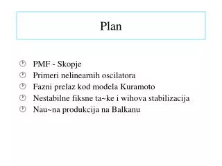
Plan
Plan. PMF - Skopje Primeri nelinearnih oscilatora Fazni prelaz kod modela Kuramoto Nestabilne fiksne ta~ke i wihova stabilizacija Nau~na produkcija na Balkanu. PMF, Skopje. Prose~na golemina na evropski oddel za fizika (2009).

Plan
E N D
Presentation Transcript
Plan PMF - Skopje Primeri nelinearnih oscilatora Fazni prelaz kod modela Kuramoto Nestabilne fiksne ta~ke i wihova stabilizacija Nau~na produkcija na Balkanu
Prose~na golemina na evropski oddel za fizika (2009) Studenti - 467 (univerzitet - 23260) Nastaven personal - 79 (univ - 1990) Doktoranti - 75 Na PMF, soodvetno st. 20-30, n. 23 i d. 7-8 . . .
Current programme – part 1(semesters 1-4) (lectures + tutorials + laboratory = credit points) I II Mechanics 4+2+2=8 Molecular physics 4+2+2=8 Mathematical Analysis 1 4+4+0=8 Mathematical analysis 2 3+3+0=7 Computer usage in physics 2+0+2=4 Chemistry 3+0+3=6 Introduction to metrology 2+0+2=4Elective course 3 3+0+0=3 Elective course 1 3+0+0=3 Elective course 4 3+0+0=3 Elective course 2 3+0+0=3 Elective course 5 3+0+0=3 III IV Electromagnetism 4+2+2=7 Optics 4+2+2=8 Mathematical physics 1 3+3+0=7 Mathematical physics 2 3+3+0=7 Theoretical mechanics 3+2+0=6 Electronics 3+1+3=7 Oscillations and waves 2+2+0=4 Theoretical electrodynamics and Elective course 6 3+0+0=3 special theory of relativity 3+2+0=5 Elective course 7 3+0+0=3 Elective course 8 3+0+0=3
Current programme - part 2(semesters 5-8, physics teachers branch) V VI Atomic physics 4+2+2=8 Nuclear physics 4+2+2=8 Measurements in physics 3+0+3=6 Introduction to quantum theory 3+2+0=6 General astronomy 2+1+0=4Introduction to materials 2+0+2=5 Elective course 9 3+0+0=3Basics of solid state physics 3+1+2=6 Elective course 10 3+0+0=3 Pedagogy 3+2+0=5 Elective course 11 3+0+0=3 Elective course 12 3+0+0=3 VII VIII Use of computers in teaching 2+0+2=5Methodology of physics teaching 2 Methodology of physics teaching 1 2+2+3=8 (school practice)2+2+3=8 School experiments 1 2+0+3=6 School experiments 2 2+0+3=5 Psychology 3+2+0=5 Design of electronic equipment 2+0+3=4 Macedonian language 0+2+0=2 History and philosophy of physics 3+1+0=4 Introduction to biophysics 2+0+2=4 Diploma thesis 0+0+9=9
The Lorenz system E. N. Lorenz, “Deterministic nonperiodic flow,” J. Atmos. Sci. 20 (1963) 130. Fixed points: C0 (0,0,0) C± (±8.485, ±8.485,27) Eigenvalues: l(C0) = {-22.83, 11.83, -2.67} l(C±) = {-13.85, 0.09+10.19i, 0.09-10.19i} Chaotic attractor of the unperturbed system (F(t)=0)
Historical example from Biology The glowworms ... Represent another shew, which settle on some Trees, like a fiery cloud, with this surprising circumstance, that a whole swarm of these insects, having taken possession of one Tree, and spread themselves over its branches, sometimes hide their Light all at once, and a moment after make it appear again with the utmost regularity and exactness … Engelbert Kaempfer description from his trip in Siam (1680)
Further examples • The Moon facing the Earth; Gallilean satelites; Kirkwood gaps • Cyclotron and other accelerators • Stroboscope; Fax-machine • Biological clocks; Jet lag • Pacemakers • Farmacological actions of steroids
Further examples 2 • Cardiorespiratory system • Entrainment of cardial and locomotor rhythms • Cardiovascular coupling during anesthesia • Synchronization between parts of the brain • Magnetoencephalographic fields and muscle activity of Parkinsonian patients
Parametar na poredok i sinhronizacija
Re{enie na modelot na Kuramoto (1975) re{enija i
INTRODUCTION - THE PYRAGAS CONTROL METHOD - Time-delayed feedback control (TDFC) - Time-delayed autosynchronization (TDAS) K. Pyragas, Phys. Lett. A 170 (1992) 421
Applications Delays are natural in many systems • Coupled oscillators • Electronic circuits • Lasers, electrochemistry • Networks of oscillators • Brain and cardiac dynamics
VARIABLE DELAY FEEDBACK CONTROL OF USS Pyragas control force: - noninvasive for USS and periodic orbits VDFC force: - piezoelements, noise - saw tooth wave: - random wave: - sine wave: A. Gjurchinovski and V. Urumov – Europhys. Lett. 84, 40013 (2008)
THE MECHANISM OF VDFC 2D UNSTABLE FOCUS WITH A DIAGONAL COUPLING n – sufficiently large original system : comparison system : Characteristic equation of the comparison system (2D focus):
THE MECHANISM OF VDFC TDAS VDFC VDFC VDFC
THE MECHANISM OF VDFC The effect of including variable delay into TDAS for small e • condition for the roots lying on the imaginary axis for e=0 to move to • the left half-plane as e increases from zero CONCLUSION: the stability domain will expand in all directions within the half-space K>K0, as soon as e is increased from zero, independent of the precise way in which the delay is varied
THE MECHANISM OF VDFC 2D unstable focus with l = 0.1 and w = p e = 0 (Pyragas) Increase of the stability domain for small e > 0 e = 0 (brown) e = 0.07 (green) e = 0.1 (yellow)
THE MECHANISM OF VDFC e-Kdiagrams for a saw tooth wave modulation (T0=1)
THE MECHANISM OF VDFC Stability analysis for the Lorenz system (saw tooth wave) C0 (0,0,0) C+ (8.485, 8.485,27) C- (-8.485, -8.485,27) s = 10, r = 28, b = 8/3
THE MECHANISM OF VDFC The Rössler system (sawtooth wave) e = 0 e = 0.5 e = 1 e = 2 O.E. Rössler, Phys. Lett. A 57, 397 (1976). Fixed points: C1 (0.007,-0.035,0.035) C2 (5.693, -28.465,28.465) Eigenvalues: l(C1) = {-5.687,0.097+0.995i,0.097-0.995i} l(C2) = {0.192,-0.00000459+5.428i, -0.00000459-5.428i}
T(t) T(t) 2T0 2T0 T0 T0 4t t t 2t 2t 3t 4t 3t t t K(t) K K/2 4t t 2t 3t t STABILIZATION OF UPO BY VDFC • SQUARE WAVE MODULATION • periodic change of the delay, e. g. between T0 and 2T0, K fixed (VDFC) • periodic change of the delay, K varied (VDFC + SCHUSTER, STEMMLER) • - half-period of the wave (optimal choice: t=T0) +
STABILIZATION OF UPO BY VDFC RösslerT0=5.88 • PYRAGAS F(t)=K [y(t-T0)-y(t)] • VDFC (square wave) F(t)=K [y(t-T(t))-y(t)] • SCHUSTER, STEMMLER F(t)=K(t) [y(t-T0)-y(t)] • VDFC (square wave) + SCH-ST F(t)=K(t) [y(t-T(t))-y(t)]
STABILIZATION OF UPO BY VDFC RösslerT0=17.5 RösslerT0=11.75
STABILIZATION OF UPO BY VDFC K periodically varied between K and K/4 (Rössler, T0=17.5) • VDFC + SCHUSTER • Restricted VDFC + SCHUSTER F(t)=K(t) Sin [y(t-T(t))-y(t)]
STABILIZATION OF UPO BY VDFC Rössler T0=5.88 VDFC (square wave) t = T0 t = 2T0 t = T0/2
STABILITY ANALYSIS - RDDE Retarded delay-differential equations • GOAL:stabilization of unstable steady states by a variable-delay feedback control in a nonlinear dynamical systems described by a scalar autonomous retarded delay-differential equation (RDDE) • MOTIVATION:extension of the delay method to infinite dimensional systems • INTEREST:frequent occurrence of scalar RDDE in numerous physical, biological and engineering models, where the time-delays are natural manifestation of the system’s dynamics T. Erneux, Applied Delay Differential Equations (Springer, New York, 2009)
DELAY-DIFFERENTIAL EQUATIONS Retarded delay-differential equations General scalar RDDE system: T1≥ 0 – constant delay time F – arbitrary nonlinear function of the state variable x Linearized system around the fixed point x*: Characteristic equation for the stability of steady state x* of the free-running system: A. Gjurchinovski and V. Urumov – Phys. Rev. E 81, 016209 (2010)
STABILITY ANALYSIS - RDDE Retarded delay-differential equations Controlled RDDE system: u(t) – Pyragas-type feedback force with a variable time delay K – feedback gain (strength of the feedback) T2 – nominal delay value f– periodic function with zero mean – amplitude of the modulation – frequency of the modulation
STABILITY ANALYSIS - RDDE Stability of the unperturbed system
STABILITY ANALYSIS - RDDE Stability under variable-delay feedback control Limitation of the VDFC for RDDE systems: • A kind of analogue to the odd-number limitation in the case of delayed feedback control of systems described by ordinary differential equations: • W. Just et al., Phys. Rev. Lett. 78, 203(1997) • H. Nakajima, Phys. Lett. A 232, 207 (1997) • … refuted recently: • B. Fiedler et al., Phys. Rev. Lett. 98, 114101 (2007). • B. Fiedler et al., Phys. Rev. E 77, 066207 (2008).
STABILITY ANALYSIS - RDDE Representation of the control boundaries parametrized by = Im() (K,T2) plane:
EXAMPLES AND SIMULATIONS Mackey-Glass system • A model for regeneration of blood cells in patients with leukemia • M. C. Mackey and L. Glass, Science 197, 28 (1977). • M-G system under variable-delay feedback control: • For the typical valuesa = 0.2, b = 0.1 and c = 10, the fixed points of the free-running system are: • x1 = 0 – unstable for any T1, cannot be stabilized by VDFC • x2 = +1 – stable for T1 [0,4.7082) • x3 = -1 – stable for T1 [0,4.7082)
EXAMPLES AND SIMULATIONS Mackey-Glass system (without control) • T1 = 4 • T1 = 8 • T1 = 15 • T1 = 23
EXAMPLES AND SIMULATIONS Mackey-Glass system (VDFC) T1 = 23 • = 0 (TDFC) • = 0.5 (saw) • = 1 (saw) • = 2 (saw)