Download
1 / 21
210 likes | 235 Vues
Explore real-time image processing and robotics in automotive applications, driver assistance, collision warning systems, and more. Simulate car traffic flow based on physics laws with position, speed, and cruising parameters. Utilize road utilization data for analysis and visualization.

E N D
Contents • Introduction & Motivation • Environment Modeling (Roadways) • Simulation • Statistics • Visualization • Conclusion
Introduction • Real-time image processing and Robotics for automotive applications • Driver assistance using Intelligent feedback on traffic conditions, cross-roads accidents, etc. • Collision warning and avoidance system • Intelligent parking assistance
Environment Modeling- Roadways • Preparing the map The map is stored in a text file • It is represented by: • Lines • Curves
Representing lines • ( x1, y1, z1 ) -> ( x2, y2, z2 ) line 125 400 10 125 375 20
Representing curves • ( x, y, z, r, anglestart, anglestop, direction) arc 125 300 20 75 270 180 -1
Sampling • Sampling distance • Line • length of line • number of sampling points • allocating the points • Curve • angle • length of arc • number of sampling points • angle of sampling points • allocating the points
Simulation of Car Traffic Flow • Based on physics laws (kinematics) • The control parameters: • the number of cars • the size of the histogram interval (for generating statistics) • Equations • the velocity law: • the position law:
The parameters of the cars • Position on the road: index and lane • Current speed and cruising speed • Maximum acceleration • Maximum deceleration • Reaction time of the driver
How the simulation works • The time is divided into small intervals (~ 10ms) • In one time slice a car can only: • maintain speed • accelerate • decelerate
The algorithm • for each car • must decelerate ? • yes: decelerate ! • no: current speed < cruising speed & can accelerate ? • yes: accelerate ! • no: maintain speed.
When the car must decelerate ? • We search for the cars in front of the current car • When the cars in front of the current car are close together (20m), they block the road. • We assume that in the next time-slice the cars in front will maintain speed (a reasonable assumption) • After that, we check if we maintain the speed of the current car, the time distance between cars will be decreasedbelow the time_dist (a constant value).
The car can accelerate? • a car can accelerate when the time distance to the car in front is less than the time_distanceor when an overtake is performed (not yet implemented) • the maximum allowed acceleration is the greatest between the maximum possible acceleration of the car and the acceleration that will not lower the time distance under time_distance
Acceleration and Deceleration • We update the position and the velocity:
Utilization of road • Dividing the road to smaller intervals • Counting the number of cars on each interval -> histogram • Drawing a chartminimal, average, maximal utilization
3D Visualization • Actually a 2.5D representation • It can be rotated and zoomed in and out • Still to do more !!