Download
1 / 43
450 likes | 841 Vues
INTRODUCTION TO DISCHARGE RATING CURVES. ‘Hydrographic Basics’ Training May 2011. What is a ‘Control’?. “The physical element or combination of elements that controls the stage-discharge relation”. ‘Natural’ Controls. ‘Natural’ Controls. Stable and sensitive control.

E N D
INTRODUCTION TO DISCHARGE RATING CURVES ‘Hydrographic Basics’ Training May 2011
What is a ‘Control’? “The physical element or combination of elements that controls the stage-discharge relation”
‘Natural’ Controls Stable and sensitive control Control enhanced to improve sensitivity
‘Natural’ Controls Broad and insensitive Control Unstable control
‘Artificial’ Controls – Thin Plate Weirs ‘V’-Notch Cipolletti
‘Artificial’ Controls–Compound Weirs Sharp crested compound gauging weir with dividing walls between notches Sharp crested compound gauging weir without dividing walls Sharp crested compound gauging weir with aeration piers between notches
‘Artificial’ Controls–Compound Weirs Sharp crested compound gauging weir with dividing walls between notches Horizontal Crump (triangular) compound gauging weir with dividing walls between notches
Weir and Flume Combination Sharp crest/Hydro flume combination gauging weir
What is a Discharge Rating? Discharge Rating is a function of the downstream physical features of the stream – i.e. the ‘control’ Relates gauge height (i.e. stage) and discharge (i.e. flow) Allows discharge to be estimated at any gauge height Non-linear at some gauge heights (e.g. backwater effects, hysteresis) Required constant verification – over a wide range of gauge heights Can be estimated from mathematical formulae (normally for ‘man-made’ structures such as weirs & flumes)
Why Do We Need Gaugings? Shifting and changes to control Changes in downstream channel physical features (e.g. vegetation) Backwater effects Channel bank instability Channel scouring
Continuity Equation Q = A * V Where: Q = Discharge (flow) A = Cross-sectional area V = Mean Velocity
Rating VerificationVarious Gauging Methods Volumetric Wading Boat Float Bridge Cableway – manned Cableway – un-manned Dyes (e.g. rhodamine) Chemicals (e.g. sodium chloride)
Rating Curve DerivationGeneral Equation Method Mathematical Formulae Limited to ‘special design’ controls (e.g.: V-notch, broad crested rectangular weirs) Not suitable for complex control structures (e.g.: natural controls)
Rating Curve DerivationLinear Plot Method Gauge Height (GH) plotted on vertical axis Discharge (flow) plotted on horizontal axis Parabolic curve concave ‘downwards’ Low, medium and high flow curves plotted Effects of irregular stream cross-sections
Linear Curve MethodAdvantages Allows hydrographer to quickly identify changes in stream discharge rating Downstream effects on rating easily identified Identifies different control effects throughout flow range
Linear Curve MethodDisadvantages Rating curve extensions not easily undertaken
Rating Curve DerivationLogarithmic Plot Method ‘Gauge Height’ minus ‘Cease to Flow’ value plotted on vertical axis Discharge (flow) plotted on horizontal axis Plotted on log-log paper Discharge curve plots as a ‘straight line’ Natural streams – logarithmic curve rarely a straight line over entire flow range (e.g.: irregular cross-sections, downstream features, ‘overbank’ flow) A number of ‘change points’ evident
Include Velocity Head Rating Curve DerivationDetermination of CTF Gauge Pool Control Section Flow Deepest Point on Control Gauge Pool Control Section Perpendicular to Flow
Logarithmic Curve MethodAdvantages Facilitates an ‘easy’ method of curve extension (for BOTH low and high flow regimes) Gauging deviation from curve easily identified (straight line analysis) Highlights changes in stream cross-section and control changes throughout flow range (change points)
Logarithmic Curve MethodDisadvantages Gauge Height scale too open in LOW flow regime Gauge Height scale too compressed in HIGH flow regime
Rating Curve Development • Determine ‘Cease to Flow’ point • Minimum of 10-12 ‘well spaced’ gaugings required • Plot gaugings to BOTH linear and logarithmic curves • Rising GH gaugings plot to the ‘right’ of the curve, falling gaugings tend to plot to the ‘left’ of the curve • Compute gaugings on site (if >5% deviation from current curve, second gauging should be taken at an alternate section of the stream) • Determine ‘Period of Applicability’ • Cross-sections at control, orifice and cableway required immediately AFTER floods • Regular gauging required over a ‘wide’ range of Gauge Heights • Ongoing monitoring of site required (i.e.: visual observation, gauging, survey) Rating table changes and re-issues should be approved by a suitably qualified and experienced person
Rating Curve Extrapolation (When?) Required when range required for computation is outside range of ‘gauged’ flows Likely causes are: - control change - scouring of bed - backwater effects - change in downstream stream geometry
Rating Curve Extrapolation (How?) Recommended that more than one method used Main methods are: - Logarithmic extension - Gauge Height - Velocity - Stevens Method (A√d) - Manning's Formula
Logarithmic Method A rating curve plotted on log-log coordinates will plot as a straight line Q = K (GH - ctf)↑n Where Q = discharge K = a constant GH = Gauge Height ctf = Cease to flow GH n = a function of the shape of the cross-section
Logarithmic Method · · · Depth above CTF Change Point 2 · Change Point 1 · · · · = gauging Discharge
Logarithmic Method • If the log-log extension exceeds the maximum measured flow by approximately 20%, other methods such as Mannings or velocity – area should be used.
Velocity - Area Method Based on ‘Continuity Equation’ Q = A V Where Q = Discharge A = Cross-sectional area V = Mean velocity Requires an accurate cross-section surveyed up to the highest gauge height required for the rating extension Area can be plotted against gauge height and an area for any gauge height can be determined Mean velocity of the stream is derived directly from gauging results (provided gaugings are taken at the prime gauge section) The mean velocity is plotted against the gauge height At higher stages the rate of increase in the velocity through the measurement section will diminish rapidly. The Gauge height-Velocity curve is then extended to the desired stage Discharge then computed from product of Area and Velocity
Stevens (or A√d ) Method Requires an accurate cross-section Should not be used where ‘over-bank’ flow conditions exist Has little value for extrapolation of curve to cover lower flow regime Based on an adaption of ‘Chezy’s Formula’ Q = KA√d Where Q = Discharge K = a constant A = Cross-sectional area (from cross-section) d = mean depth at cross-section (area / width) ‘Q’ and ‘GH’ are each plotted against A*√d (straight line which is extended) This will plot as a straight line which can be extended to extrapolate discharge above maximum recorded GH
MANNINGS FORMULA Requires an accurate cross-section Should not be used where ‘overbank’ flow conditions exist Based on Manning's Formula: Q = A (r↑0.6667) √s n Where Q = Discharge A = Cross-sectional area (from cross-section) r = hydraulic radius (area/wetted perimeter) s = slope n = Manning’s n* As √s becomes constant at higher gauge heights, the formula becomes: n V = k(r↑0.6667) Where: V = Mean velocity k = constant r = hydraulic radius (area/wetted perimeter) * Can range from 0.010 (smooth concrete banks) to 0.035 (weedy banks)
Mannings Formula(continued) As ‘r’ can be computed from cross-sections, ‘V’ can be taken from the GH-Velocity curve, ‘k’ can be computed from the above equation When ‘k’ is plotted against GH the curve should reach a constant value at higher stages This straight line portion may be extended to give the value of ‘k’
Manning’s Formula(continued) • Straight reach of channel should be at least 60m in length, free of rapids, abrupt falls and sudden contractions and expansions • Slope is determined by dividing the difference in water surface level at the start and finish of the reach by the length of the reach • Hydraulic radius is the area of the cross-section divided by the wetted perimeter • The Mannings co-efficient of roughness is dependent on characteristics of channel and can be derived from following table: