Download

1 / 90
910 likes | 1.08k Vues
IVW Cursus 7 Oktober 2003 Betrouwbaarheid van systemen en elementen. Pieter van Gelder TU Delft. Inhoud. Tijdsafhankelijke faalkansen Faalkansberekening op systeem niveau Parallel en serieel Afhankelijkheden Faalkansberekening op element niveau Niveau III, II, en I. 1. 0.8. P(X x ).

E N D
IVW Cursus7 Oktober 2003Betrouwbaarheid van systemen en elementen Pieter van Gelder TU Delft
Inhoud • Tijdsafhankelijke faalkansen • Faalkansberekening op systeem niveau • Parallel en serieel • Afhankelijkheden • Faalkansberekening op element niveau • Niveau III, II, en I
1 0.8 P(Xx) 0.6 (x) X F 0.4 0.2 0 x 0.5 0.4 P(x < X x+d x) 0.3 fX(x) 0.2 0.1 0 x x+d x
J.K. Vrijling and P.H.A.J.M. van Gelder, The effect of inherent uncertainty in time and space on the reliability of flood protection, ESREL'98: European Safety and Reliability Conference 1998, pp.451-456, 16 - 19 June 1998, Trondheim, Norway.
T = time to failure • The Hazard Rate, or instantaneous failure rate is defined as: • h(t) = f(t) / [1 - F(t) ] = f(t) / R(t) • f(t) probability density function of time to failure, • F(t) is the Cumulative Distribution Function (CDF) of time to failure, • R(t) is the Reliability function (CCDF of time to failure). • From: f(t) = d F(t)/dt , it follows that: • h(t) dt = d F(t) / [1 - F(t) ] = - d R(t) / R(t) = - d ln R(t)
Integrating this expression between 0 and T yields an expression relating the Reliability function R(t) and the Hazard Rate h(t):
Constant Hazard Rate • The most simple Hazard Rate model is to assume that: h(t) = λ , a constant. This implies that the Hazard or failure rate is not significantly increasing with component age. Such a model is perfectly suitable for modeling component hazard during its useful lifetime. • Substituting the assumption of constant failure rate into the expression for the Reliability yields: • R(t) = 1 - F(t) = exp (- λt) • This results in the simple exponential probability law for the Reliability function.
Non-Constant Hazard Rate • One of the more common non-constant Hazard Rate models used for evaluation of component aging phenomenon, is to assume a Weibull distribution for the time to failure: • Using the definition of the Hazard function and substituting in appropriate Weibull distribution terms yields: • h(t) = f(t) / [1 - F(t) ] = β t β -1 / t β
For the specific case of: β = 1.0 , the Hazard Rate h(t)reverts back to the constant failure rate model described above, with: t = 1/ λ . The specific value of the β parameter determines whether the hazard is increasing or decreasing.
Effect of inherent uncertainty on decrease in hazard rate • Example: PAC dike and sea dike
Reliability Reliability is the probability that a process or a system will operate without failure for a given period and under given operating conditions. R(t) = e-lt This equation is the exponential reliability function, it applies only for cases of “constant failure rate”, where l is failure rate.
Maintainability Maintainability is the probability that a process or a system that has failed will be restored to operation effectiveness within a given time. M(t) = 1 - e-mt where m is repair (restoration) rate
The Concept of Availability Reliability Maintainability Availability
Availability Availability is the proportion of the process or system “Up-Time” to the total time (Up + Down) over a long period. Up-Time Up-Time + Down-Time Availability =
Process Requirements Process Effectiveness Capability Performance Availability Reliability Maintainability Dependability
Capability: A measure of the ability of a process to satisfy given requirements (A measure of Quality - no time dependency) Availability: A measure of the ability of a process to complete a mission without excessive down time (Depends on Reliability and Maintainability) Dependability: A measure of the ability of a process to commence and complete a mission without failure (Depends on Reliability and Maintainability)
System Operational States B1 B2 B3 Up t Down A1 A2 A3 Up: System up and running Down: System under repair
Mean Time To Fail (MTTF) MTTF is defined as the mean time of the occurrence of the first failure after entering service. B1 + B2 + B3 3 MTTF = B1 B2 B3 Up t Down A1 A2 A3
Mean Time Between Failure (MTBF) MTBF is defined as the mean time between successive failures. (A1 + B1) + (A2 + B2) + (A3 + B3) 3 MTBF = B1 B2 B3 Up t Down A1 A2 A3
Mean Time To Repair (MTTR) MTTR is defined as the mean time of restoring a process or system to operation condition. A1 + A2 + A3 3 MTTR = B1 B2 B3 Up t Down A1 A2 A3
Availability Availability is defined as: Up-Time Up-Time + Down-Time A = Availability is normally expressed in terms of MTBF and MTTR as: MTBF MTBF + MTTR A =
Reliability/Maintainability Measures Reliability R(t) (Failure Rate) l = 1 / MTBF R(t) = e-lt Maintainability M(t) (Maintenance Rate) m = 1 / MTTR M(t) = 1 - e-mt
Types of Redundancy • Active Redundancy • Standby Redundancy
Active Redundancy A Input Div Output B Divider Both A and B subsystems are operative at all times Note: the dividing device is a Series Element
Standby Redundancy A SW Input Output B Switch Standby The standby unit is not operative until a failure-sensing device senses a failure in subsystem A and switches operation to subsystem B, either automatically or through manual selection.
Series System Input A1 A2 An Output ps = p1 + p2 +……. + pn - (-1)n joint probabilities For identical and independent elements: ps ~ 1 - (1-p)n < np (>p) ps : Probability of system failure pi : Probability of component failure
Parallel System A Input Output B Multiplicative Rule ps = p1.p2 …pn ps : Probability of system failure
Haringvliet outlet sluices t t t t Time start Modellering Lifetime distribution for one component Replacement strategies of large numbers of similar components in hydraulic structures
Series / Parallel System A1 A2 Input Output C B1 B2
System with Repairs Let MTBF = q and system MTBF = qs A Input Output B For Active Redundancy (Parallel or duplicated system) qs = ( 3l + m )/ ( 2l2 ) l << m qs = m / 2l2 = MTBF2 / 2 MTTR
A SW Input Output B Switch Standby Note: The switch is a series element, neglect for now. Note: The standby system is normally inactive. For Standby Redundancy qs = ( 2l + m )/ (l2 ) qs = m / l2 = MTBF2 / MTTR
System without Repairs For systems without repairs, m = 0 For Active Redundancy qs = ( 3l + m )/ ( 2l2 ) qs = 3l / ( 2l2 ) = 3/ ( 2l) qs = (3/2) q where q = 1/l qs = 1.5 MTBF For Standby Redundancy qs = ( 2l + m )/ (l2 ) qs = 2l/ l2 = 2/ l qs = 2q where q = 1/l qs = 2 MTBF
Summary Type With Repairs Without Repairs Active MTBF2 / 2 MTTR 1.5 MTBF Standby MTBF2 / MTTR 2 MTBF Redundancy techniques are used to increase the system MTBF
R S Example: wire • Limit state function: • Z = R - S • with: variable distribution mean standarddeviation R normal 6 0 kN 5 kN S normal 4 0 kN 10 kN
Probability densities 0.08 0.07 R 0.06 0.05 S Probability density (1/N) 0.04 0.03 0.02 0.01 0 0 20 40 60 80 R,S (N)
Joint probability density 80 70 60 50 Z>0 R (kN) 40 failure: Z<0 30 20 10 0 0 20 40 60 80 S (kN)
Analytical 80 • Failure probability • Independent • R and S: 70 r dr 50 Z>0 R (kN) 40 30 falen: Z<0 20 10 0 0 20 40 r 80 S (kN)
Analytical • Elaborate: • R and S normally distributed: • Fill in and calculate
Analytical • In this case simple approach possible: • variables normally distributed • Z is linear in variables • Then Z also normally distributed. • Mean • Standard deviation