Download
1 / 45
450 likes | 630 Vues
Development and validation of the Euler-Lagrange formulation on a parallel and unstructured solver for large-eddy simulation. PhD defense: Marta Garc í a. Director: T. Poinsot & Co-director: V. Moureau. THE CONTEXT.

E N D
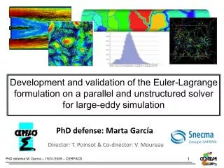
Development and validation of the Euler-Lagrange formulation on a parallel and unstructured solver for large-eddy simulation PhD defense: Marta García Director: T. Poinsot & Co-director: V. Moureau
THE CONTEXT Human nature: try to understand phenomena, comprehension effort, power of fire, energy conversion … locomotive Gas turbine This thesis is focused on the improvement of current tools to the comprehension of multiphase flows by using numerical simulation. fire • Observation • Experimentation • Numerical simulation engines
THE CONTEXT: EXPERIMENTS vs NUMERICAL SIMULATIONS EXPERIMENTS • expensive • destructives • difficult to reproduce exactly NUMERICAL SIMULATION Ham et al. Annual Research Briefs 2003 CTR Stanford Univ. • less expensive • not destructives • reproductibility Spray evolution from a realistic gas-turbine injector.
THE CONTEXT: INCREASE OF COMPUTER POWER 1012 = 1.000.000.000.000 1105x1012 Flops In the last 3 years CPU time divided by 8 (approx.) 8 weeks 1 week 280x1012 Flops 12.64x10¹² Flops 1.65x10¹² Flops(1) (1) Flops: floating point operations per second
(TPF) THE CONTEXT: TWO-PHASE FLOW NUMERICAL SIMULATION Current treatment of the dispersed phase in AVBP Eulerian formulation Lagrangian formulation ? TPF Team in 2005 … PhD PhD PhD … considering the increasing computer power and myexperienceaccumulated in the past 3 years … PhD PhD PhD PhD PhD PhD PhD PhD PhD PhD PhD PhD 2 PhD’s: CERFACS & IMFT PhDcerfacs2 Kaufmann 2004 1 PhD ??? Mossa 2005 PhDimft1 Pascaud 2006 ~ up Riber 2007 PhDcerfacs2 Boileau 2007 PhDimft1 Lamarque 2007 … Lavedrine 2008
THE CONTEXT: TWO-PHASE FLOW NUMERICAL SIMULATION Euler-Euler vs Euler-Lagrange Euler-Lagrange Euler-Euler Particle ensemble viewed as a continuous field Individual particle trajectories are computed • Easy modeling of particle movements and interactions. • Robust and accurate if enough particles are used. • Size distributions easy to describe. • Easy to implement physical phenomena (e.g. heat and mass transfer, wall-particle interaction). • Easy treatment of dense zones. • Similarity with gaseous equations. • Direct transport of Eulerian quantities. • Similarity with gaseous parallelisme. • Delicate coupling with combustion. • Difficult to run in parallel. • Each ‘particle’ actually represents an ensemble of particles. • Difficult description of polydispersion. • Difficulty of crossing sprays treatment. • Limitation of the method in very dilute zones.
THE OBJECTIVES OF THE WORK • Develop a Lagrangian formulation for two-phase flow treatment within a parallel, unstructured and hybrid solver AVBP. • Perform the first simulations on academic and complex geometries. • Verify the efficient parallel implementation to maintain good performance on massively parallel machines.
THE PLAN OF THE PRESENTATION Presentation of the simulation tool: AVBP solver Description of the Lagrangian module Application test cases: Conclusions and perspectives • Quick introduction • Domain partitioning • Rounding errors and repetitivity of LES • Particle equations of motion • Particle tracking algorithm • Decaying homogenous isotropic turbulence • Polydisperse two-phase flow of a confined bluff body
THE AVBP SOLVER • Parallel solver started in 1993. • Unstructured solver capable of handling hybrid grids of different cell types. • Computational Fluid Dynamics (CFD) code to solve laminar and turbulent compressible Navier-Stokes equationsin 2 and 3 space dimensions. • Built upon a modular software librarythat includes integrated parallel domain partition and data reordering tools, message passing (MPI) and includes supporting routines for dynamic memory allocation, routines for parallel I/O and iterative methods. • Written in standard Fortran 77 and C, but it is being upgraded to Fortran 90 in a gradual fashion. • Highly portableto different parallel machines.
THE AVBP SOLVER: PARTITIONING ALGORITHMS … currenly available in AVBP R = recursive B = bisection NODAL MESH RCB C = coordinate DUAL MESH RIB I = inertial RGB G = graph
THE AVBP SOLVER: PARTITIONING ALGORITHMS Total No of nodes CPU time of 1000 it. (s) The choice of partitioning algorithm has an effect on the CPU time of your simulation. (beforepartitioning) MESH 367,313 + 35% • Need of a new partitioning algorithm: • Faster partitioning • Lower number of total nodes after partitioning • With parallel version • With multi-constraint partitioning options • Choice done: • METIS package implemented during this thesis (after partitioning) RCB 495,232 361.5 + 37% + 1.5% RIB 503,230 366.96 + 12% + 45% RGB 530,852 405.64
THE AVBP SOLVER: PARTITIONING ALGORITHMS Some results obtained with METIS multilevel partitioning algorithm … No of nodesafter partitioning ARRIUS2_10M COMPARISON OF ALGORITHMS METIS algorithm is faster It produces a lowernumber of nodes after partitioning 4096 procs No of subdomains 29 minutes 21 minutes ARRIUS2_44M No of nodesafter partitioning No of subdomains No of subdomains
THE AVBP SOLVER: ROUNDING ERRORS … and repetitivity of LES • AVBP: Parallel solver, highly portable to solve laminar and turbulent compressible Navier-Stokes equations. Finite precision computation: lack of associativity property !! What that means … Work published in the AIAA Journal publication: AIAA Journal Vol. 46, No 7, July 2008 “Growth of Rounding Errors and Repetitivity of Large-Eddy Simulations” J.-M. Senoner, M. García, S. Mendez, G. Staffelbach, O. Vermorel and T. Poinsot CM zoom B D C A RCM MESH B A C D
THE AVBP SOLVER: ROUNDING ERRORS Axial velocity fields of a turbulent channel (TC) at different instants 4 procs Instantaneous solutions in unsteady simulations. Same initial conditions. Different number of processors. TWO NORMS ARE USED TO COMPARE RESULTS BETWEEN TWO SOLUTIONS 8 procs (t1) DIFFERENCES OBSERVED BETWEEN TWO SNAPSHOTS Axial velocity (m/s) Axial velocity (m/s) 4 procs 4 procs 8 procs 8 procs (t3) (t2) Axial velocity (m/s)
Reprinted by permission of the American Institute of Aeronautics and Astronautics. THE AVBP SOLVER: ROUNDING ERRORS Different effects observed on repetitivity of LES Norm saturation Any sufficiently turbulent flow computed in LES exhibits significant sensitivity to small perturbations, leading to instantaneous solutions which can be totally different. simple double The divergence of solutions is due to 2 combined facts: The exponentialseparation of trajectories in turbulent flows. The different propagation of roundingerrorsinduced by domainpartitioning and schedulingoperations. Machine precision differences Effect of node reordering Effect of machine precision quadruple turbulent The validation of an LES code after modifications may only be based on statistical fields. Effect of turbulence Effect of initial conditions laminar
THE PLAN OF THE PRESENTATION Presentation of the simulation tool: AVBP solver Description of the Lagrangian module Application test cases: Conclusions and perspectives • Quick introduction • Domain partitioning • Rounding errors and repetitivity of LES • Particle equations of motion • Particle tracking algorithm • Decaying homogenous isotropic turbulence • Polydisperse two-phase flow of a confined bluff body
Assumptions: Need to know the gasvelocityateachparticle location (linear interpolation) spheres [ Schiller & Nauman. 1935 ] [ Fede & Simonin 2006 ] drag + gravity The effect of the subgridfluidvelocityis not considered in thisthesis. THE LAGRANGIAN MODULE: PARTICLE EQUATIONS … of motion Individual particle trajectories are computed with a Lagrangian solver coupled to the LES code for the gas phase. N droplets to track (order of a few millions) Particlesequation of motion
Injection Locating particles in cells X3 Subdomain 1 Subdomain 2 Knowing particles positions at time n: exchange particles between processors ni ( Xp-Xi ) 0 cell i n3 Xp Two-way coupling n2 n1 influence node X1 particle X2 Particles load-balancing Interpolation algorithm gasvelocityug,iateachparticle location Particle-wall treatment THE LAGRANGIAN MODULE: KEY POINTS … for Lagrangian schemes in unstructured meshes …
2D: 3D: Face-normals: Calculation of partial volumes: X3 ni ( Xp-Xi ) 0 Xp n3 Shape functions: Xp n2 - X1 n1 + n3 n3 X2 To decide if the particle is in the cell or not, the scalar product between the vector starting from the vertex of the cell to the particle and the inward normal vector of the corresponding edge is taken. The particle is inside the cell if all the scalar products of each edge are positive. THE LAGRANGIAN MODULE: LOCATING PARTICLES … in elements of arbitrary shape
THE LAGRANGIAN MODULE: SEARCH ALGORITHMS … for different situations Search particles for the first time Search injected particles Quad/Octree Injection area Cells of the injection area Nodes of the injection area Use of different search algorithms depending on the situation to reduce memory and CPU time requirements. Particles injected F. Collino (CERFACS) Interface between processors Search particles during simulation Search particles crossing boundaries between processors Old cell containing the particle Cells surrounding the old cell Cells of the interface (type 2) Initial particle location Interface between processors New particle location Initial particle location Nodes of the containing cell New particle location
1st order Taylor Serie Ex. 1D and 1st order Linear Least Squares (LAPACK subroutine DGELS) Lagrange interpolation (only for coordinate grids with quads or hexahedras) 2 Ex. 3D with hexa: n=2 (trilinear interpolation) 1 2 2 THE LAGRANGIAN MODULE: INTERPOLATION … of gaseous-phase properties at particle position
Validation test of two-way coupling Exist an analytical solution Momentum eq. = cte 8 7 9 4 6 y 3 1 2 x THE LAGRANGIAN MODULE: TWO-WAY COUPLING … source termsand validation [ Boivinet al.1998, Boivinet al. 2000 ] [ Ph.D. O. Vermorel 2003 ] = Coupling force In the framework of PIC methods = constant of proportionality
THE LAGRANGIAN MODULE: PARTICLE INJECTION • INJECTION GEOMETRY: simple injection options available • Point injection: all droplets are injected at the same point. • Disk injection: droplets are injected over a disk. Example of input parameters: Coordinates of the injection point, disk diameter, normal to define disk direction, tolerance … • PARTICLE SIZE DISTRIBUTION: • Monodisperse: all particles have the same diameter. • Polydisperse: different particle diameters. • Gaussian distribution • Log-normal distribution Example of input parameters: Type of distribution, maximum and minimum diameters, mean and standard deviation …
z=-3mm Inject # particles by timestep THE LAGRANGIAN MODULE: PARTICLE INJECTION … example of a disk injection Injection tube ZOOM - Particle mass flow rate - Particle diameter(s), density, mean/rms velocity ...
THE PLAN OF THE PRESENTATION Presentation of the simulation tool: AVBP solver Description of the Lagrangian module Application test cases: Conclusions and perspectives • Quick introduction • Domain partitioning • Rounding errors and repetitivity of LES • Particle equations of motion • Particle tracking algorithm • Decaying homogenous isotropic turbulence • Polydisperse two-phase flow of a confined bluff body
THE APPLICATION TEST CASES Decaying Homogeneous Isotropic turbulence (HIT) • Academic test case • Well documented Polydisperse two-phase flow of a confined bluff body • Complexrecirculating flow • Large amount of data available
THE APPLICATION TEST CASES: DECAYING HIT • Simple configuration to: • Validate first developments of the Lagrangian version. • Localisation algorithms, interpolation, processor exchanges, etc.
THE APPLICATION TEST CASES: DECAYING HIT Illustration of preferential concentration Validation of particle kinetic energy results 20x103 15 Performance analysis of particle location 10 5 0 32 8 16 24
THE APPLICATION TEST CASES: CONFINED BLUFF BODY Description of the configuration Borée, J., Ishima, T. and Flour, I. 2001. The effect of mass loading and inter-particle collisions on the development of the polydispersed two-phase flow downstream of a confined bluff body. J. Fluid Mech., 443, 129-165. Work published in Journal of Computational Physics: J. Comput. Phys. Vol. 228, No 2, pp. 539-564 2009 “Evaluation of numerical strategies for large eddy simulation of particulate two-phase recirculating flows” E. Riber, V. Moureau, M. García, T. Poinsot and O. Simonin • r (m) • z (m) • EDF - R&D
THE APPLICATION TEST CASES: CONFINED BLUFF BODY Numerical parameters At the end of the presentation: study of particle load imbalance In the following: results of velocity profiles of the polydisperse simulation
THE APPLICATION TEST CASES: CONFINED BLUFF BODY Animation with AVBP-EL: gas velocity modulus with particles
Lighterparticlesrespond to the flow faster. Theirtrajectories are deviated and more influenced by turbulence. Heavierparticlespenetrate more into the recirculation bubble. THE APPLICATION TEST CASES: CONFINED BLUFF BODY Particle trajectories for the polydisperse case Particle trajectories of polydisperse case give expected results, behavior is different depending on the particle size. 20 microns 40 microns 60 microns 80 microns
20 microns 40 microns 20 int 4 int 8 int 20 int 3 mm 3 mm 10 int 16 int 16 int 10 int 12 int 4 int 12 int 8 int 60 microns 80 microns 20 int 3 mm 4 int 16 int 20 int 10 int 4 int 12 int 3 mm 16 int 8 int 10 int 12 int 8 int THE APPLICATION TEST CASES: CONFINED BLUFF BODY Cross-section velocity profiles (effect of the No of samples) ` 0.130 0.075 0.010 r (m) 3 days 12 days 45 days z (m)
Location of recirculation zone isshifted by a few mm. THE APPLICATION TEST CASES: CONFINED BLUFF BODY EXP: AVBP_EL: 0.25, 1,4 (s) Axial mean particle velocity profiles: [-2, 6] (m/s) 20 microns 40 microns 60 microns 80 microns
Minorproblem to capture the first stagnation point THE APPLICATION TEST CASES: CONFINED BLUFF BODY EXP: AVBP_EL: 0.25, 1,4 (s) Axial RMS particle velocity profiles: [0.0, 1.5] (m/s) 20 microns 40 microns 60 microns 80 microns
THE APPLICATION TEST CASES: CONFINED BLUFF BODY EXP: AVBP_EL: 0.25, 1,4 (s) Radial mean particle velocity profiles: [-1, 1] (m/s) 20 microns 40 microns 60 microns 80 microns
THE APPLICATION TEST CASES: CONFINED BLUFF BODY EXP: AVBP_EL: 0.25, 1,4 (s) Radial RMS particle velocity profiles: [0.0, 1.5] (m/s) 20 microns 40 microns 60 microns 80 microns
THE APPLICATION TEST CASES: CONFINED BLUFF BODY Important point to retain of a two-phase Lagrangian parallel simulation Gaseous phase NOT A GOOD PARALLEL SIMULATION !! Gaseous phase Dispersed phase No cells NOT A GOOD PARALLEL LAGRANGIANSIMULATION !! (A) Gaseous phase Dispersed phase A GOOD PARALLEL LAGRANGIAN SIMULATION !! No cells No particles (B)
THE APPLICATION TEST CASES: CONFINED BLUFF BODY Single-constraint (RIB) vs two-constraints (METIS) partitioning algorithm Mesh (A) RIB (B) METIS Load-balancing the disperse phase with a two-constraint partitioning algorithm improves the performance of the two-phase Lagrangian simulation edge-cut Balanced simulation (A) (B) (B) (A) Imbalanced simulation
CONCLUSIONS AND PERSPECTIVES CONCLUSIONS • The effects of rounding errors onthe repetitivity of LES was demonstrated and analysed. • An efficient implementation of a Lagrangian formulation is related to the study of partitioning algorithms, data structure, load-balancing capabilities and parallel facilities, between others. • The increase of computer poweropens a new way for two-phase Lagrangian simulations that were considered prohibitive years ago. • Validation of the Lagrangian module in an Homogeneous Isotropic Turbulence (HIT) which allows a simple analysis of several aspects of performances and particle behavior. • A more complete study and validation has been done in a particle-laden bluff-body configuration. Results are in good agreement with experiments. Feasibility demonstrated of load-balancing capabilities.
CONCLUSIONS AND PERSPECTIVES PERSPECTIVES • Modeling • Evaporation model (Ph.D. F. Jaegle). • Treatment of particle-wall interactions (Ph.D. F. Jaegle). • Improvement of particle injection (Ph.D. J.M. Senoner+ C. Habchi IFP). • Introduction of collision and coalescence models. • Introduction of subgrid-scale fluid velocity on particle components. • Numerics • Improvement of searching algorithms and data structure. • Improve analysis of current performances: communications, algorithms, memory requirements, etc.
Thank you for your attention ! Any question ?
THE AVBP SOLVER: PARTITIONING ALGORITHMS Effect of different partitioning algorithms on CPU time ARRIUS2_44M with RCB: 0.5 [hours] * 4096 [processors] * 0.2 [euros/processor/hour] = 409.6 euros !! SAME ALGORITHM, DIFFERENT MESHES SAME MESH, DIFFERENT ALGORITHMS RIB • Need of a new partitioning algorithm: • Faster partitioning • Less number of total nodes after partitioning • With parallel version • With multi-constraint partitioning options • Choice done: METIS package 4.7 hours; 4096 procs
THE AVBP SOLVER: ROUNDING ERRORS The representation of numbers (71)10 = 7x 101 + 1x 100 decimal binary (1000111)2 = 1x 26 + 0x 25 + 0x 24 + 0x 23 + 1x 22 + 1x 21 + 1x 20 binary (real) (5.5)10 = (101.1)2 = 1x 22 + 0x21 + 1x 20 + 1x 2-1 -1/2 1/2 0.1 Numbers represented in a line 0 -2 1 2 -1 zoom A+D’=B A+D=C … B A C A+ A- B+ C- C+ B-
THE APPLICATION TEST CASES: CONFINED BLUFF BODY Single-constraint (RIB) vs two-constraints (METIS) partitioning algorithm Mesh (A) RIB (B) METIS Load-balancing the disperse phase with a two-constraint partitioning algorithm improves the performance of the two-phase Lagrangian simulation edge-cut (A) Good speedup (B) (B) (A) Bad speedup