Download
1 / 18
180 likes | 197 Vues
Explore the impact of polarization on retrievals in the Orbiting Carbon Observatory mission, focusing on CO2 levels to understand climate change patterns. Investigate the role of oceans and land ecosystems in absorbing CO2, the Northern Hemisphere land sink, and factors influencing carbon sinks. Discover how CO2 flux inversion capabilities can provide accurate data for global climate predictions through remote sensing retrievals and high-resolution spectroscopic measurements. Gain insights into radiative transfer essentials and sensitivity analyses to optimize CO2 retrieval strategies.

E N D
The Orbiting Carbon Observatory Mission: Effects of Polarization on Retrievals Vijay Natraj Advisor: Yuk Yung Collaborators: Robert Spurr (RT Solutions, Inc.), Hartmut Boesch (JPL), Yibo Jiang (JPL)
Outline • Introduction • Retrieval Strategy • Radiative Transfer Essentials • O2 A Band Results • Sensitivity Analysis • Outlook
Introduction Since 1860, global mean surface temperature has risen ~1.0 °C with a very abrupt increase since 1980. Atmospheric levels of CO2 have risen from ~ 270 ppm in 1860 to ~370 ppm today. Does increasing atmospheric CO2 drive increases in global temperature? Do increasing temperatures increase atmospheric CO2 levels?
Where are the Missing Carbon Sinks? • Only half of the CO2 released into the atmosphere since 1970 has remained there. The rest has been absorbed by land ecosystems and oceans • What are the relative roles of the oceans and land ecosystems in absorbing CO2? • Is there a northern hemisphere land sink? • What are the relative roles of North America and Eurasia? • What controls carbon sinks? • Why does the atmospheric buildup vary with uniform emission rates? • How will sinks respond to climate change? • Reliable climate predictions require an improved understanding of CO2 sinks • Future atmospheric CO2 increases • Their contributions to global change
Why Measure CO2 from Space?Improved CO2 Flux Inversion Capabilities • Current State of Knowledge • Global maps of carbon flux errors for 26 continent/ocean-basin-sized zones retrieved from inversion studies • Studies using data from the 56 GV-CO2 stations • Flux residuals exceed 1 GtC/yr in some zones • Network is too sparse • Inversion tests • global XCO2 pseudo-data with 1 ppm accuracy • flux errors reduced to <0.5 GtC/yr/zone for all zones • Global flux error reduced by a factor of ~3. Flux Retrieval Error GtC/yr/zone Rayner & O’Brien, Geophys. Res. Lett. 28, 175 (2001)
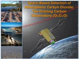
OCO Mission • First global, space-based observations of atmospheric CO2 • high accuracy, resolution and coverage • geographic distribution of CO2 sources and sinks and variability • High resolution spectroscopic measurements of reflected sunlight • NIR CO2 and O2 bands • Remote sensing retrieval algorithms • estimates of column-averaged CO2 dry air mole fraction (XCO2) • accuracies near 0.3% (1 ppm) • Chemical transport models • spatial distribution of CO2 sources and sinks • two annual cycles
Spectroscopy • Column-integrated CO2 abundance => Maximum contribution from surface • High resolution spectroscopic measurements of reflected sunlight in near IR CO2 and O2 bands O2A band Clouds/Aerosols, Surface Pressure “weak” CO2 band Column CO2 “strong” CO2 band Clouds/Aerosols, H2O, Temperature
Radiative Transfer Essentials Fundamental Equation of RT Beer’s Law Source Function (Emission, Scattering)
Polarization and the Stokes Vector • Electromagnetic radiation can be described in terms of the Stokes Vectors: I, Q, U & V • I - total intensity • Q & U - linear polarization • V - circular polarization • Degree of Polarization (for OCO)
Atmospheric and Surface Setup • 11-layer plane-parallel atmosphere (4 in stratosphere) • Urban, tropospheric and stratospheric aerosols • Lambertian surface: albedos of 0.05, 0.1, 0.3 • SZA: 10°, 40°, 70° • VZA: 0°, 35°, 70° • Azimuth: 0°, 45°, 90°, 135°, 180° • Aerosol extinction optical depth: 0, 0.025, 0.25
Results for O2 A Band with Rayleigh Scattering 0.0113 0.818 103.539
Linear Sensitivity Analysis • Park Falls, Wisconsin • Geometry • Nadir viewing • SZA: 75.1° (Jan), 34.8° (Jul) • Azimuth: 210.9° (Jan), 240.0° (Jul) • Lorentzian ILS • Resolving Powers • O2A Band: 17000 • CO2 Bands: 20000 • Errors • July: 0.3 ppm • January: 10 ppm
Outlook • Polarization: significant part of retrieval error budget • Full vector retrieval too time-consuming and not practical • Ways to handle polarization? • Orders of Scattering • Spectral Binning • Look-up tables