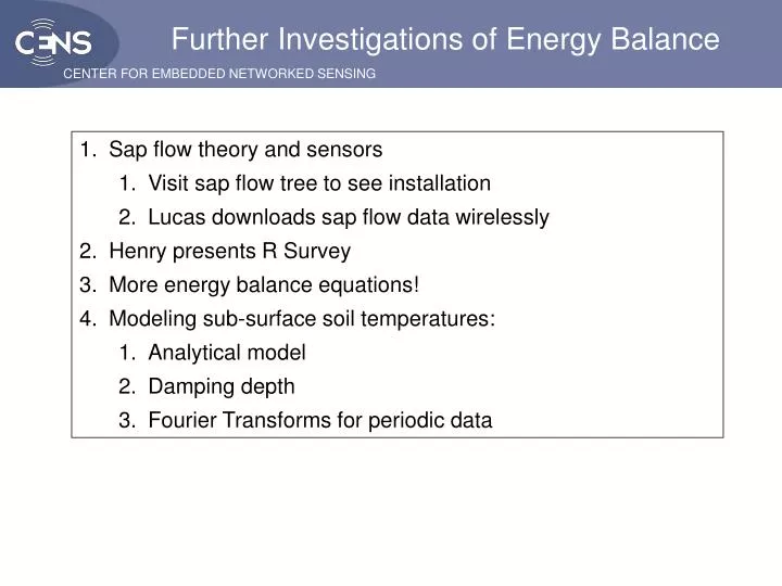
Further Investigations of Energy Balance

1. Further Investigations of Energy Balance • Sap flow theory and sensors • Visit sap flow tree to see installation • Lucas downloads sap flow data wirelessly • Henry presents R Survey • More energy balance equations! • Modeling sub-surface soil temperatures: • Analytical model • Damping depth • Fourier Transforms for periodic data

2. Science Motivation Being able to model and predict sub-surface soil temperatures will allow us to better understand the interactions of temperature with the biological components of the soil. For instance: • CO2 fluxes that are observed in forest soil environments are spatially and temporally heterogeneous and are difficult to predict, influencing estimates of total carbon fluxes of forests (Davidson et al. 1998; Trumbore 2006). • Thermal environments in soils along costal areas influence the composition of algae, plant, and animal communities (Whitecraft and Levin 2007; Bortolus et al., 2002)

3. Science Motivation Surface measurements are much more easy to conduct than sub-surface measurements with buried probes. Because the soil surface temperature depends on periodic energy inputs, we should be able to measure a few parameters, then calculate the soil temperatures at depth using a Fourier series and an analytical model. A Fourier series decomposes a periodic function or periodic signal into a sum of simple sines and cosines. “Fourier series were introduced by Joseph Fourier (1768–1830) for the purpose of solving the heat equation in a metal plate. It led to a revolution in mathematics…”

4. Soil Energy Balance Net radiation − Stored heat flux − Sensible heat flux = Latent heat flux (solar) (change in temp) (air/water) (evaporation) (Rn) (G) (H) (L)

5. Soil Temperature Soil temperatures decrease in amplitude and shift in time with depth. Different locations with different solar input (shading) will have different water content and soil characteristics. These differences will result in different “damping depths”, the parameter that describes the attenuation and delay of the daily temperature peak.

6. First Approximation – a sine wave

7. Modeling Sub-surface Temperatures

8. z is the depth at which we want to model temperature. • is the average temperature at the surface • is the amplitude of the temperature fluctuation • d is the damping depth • t is the time • p is the period • tmax is the time at which the surface temperature wave is at its maximum. Modeling Sub-surface Temperatures

9. z is the depth at which we want to model temperature. • is the average temperature at the surface • is the amplitude of the temperature fluctuation • d is the damping depth • t is the time • p is the period • tmax is the time at which the surface temperature wave is at its maximum. Modeling Sub-surface Temperatures

10. Decrease in amplitude (damping) Phase shift (delay) Modeling Sub-surface Temperatures Calculating damping depth based on decrease in amplitude and phase shifts

11. Modeling Sub-surface Temperatures Calculating damping depth based on decrease in amplitude and phase shifts

12. Modeling Sub-surface Temperatures Damping depth can also be calculated from soil physical properties. Example here is dry soil from a temperate forest. Damping depth is related to frequency of the temperature pulse ( = 2π/period) and:  = thermal conductivity C = volumetric heat capacity  = thermal diffusivity Thus, for a 86400 s period and damping depth of 15 cm,  = 8 × 10-7 m2 s-1.

13. Modeling Sub-surface Temperatures • Damping depth can also be calculated from soil physical properties. • Example here is dry soil from a temperate forest. • Damping depth is related to frequency of the temperature pulse ( = 2π/period) and: • = thermal conductivity (W m-1 °C) • C = volumetric heat capacity • (MJ m-3 °C-1) • = thermal diffusivity (10-7 m2 s-1) Thus, for sand, d = 3.56 cm

14. Modeling Sub-surface Temperatures Damping depth can also be calculated from a finite difference equation, provided enough data: Example sine waves (time interval is 0.5 minutes between temperature readings). n is the sequential measurement and j is the depth of that measurement. Use R to fit the data to the model (we will fit data to a model a little later). Parameters: Estimate Std. Error t value Pr(>|t|)  = 7.796e-06 7.939e-09 982 <2e-16 *** d = 14.64 cm

15. Fourier Transforms Fourier frequency decomposition. A Fourier transform will take a signal and decompose it into a series of superimposed sine waves, each with a shorter period (higher frequency) and each with a magnitude that determines the sine wave’s influence on the original signal.

16. Fourier Transforms

17. Fourier Transforms

18. Fourier Transforms

19. PASI Soil Temperature Exercise #1 Practice with one year of soil temperature data from Puerto Cuatreros, provided by Cintia. • Look at some built-in R time series functions. • Explore some visualizations in R. • Fourier Transform the data near the surface and reconstruct the temperature signal for a check of the method. • Estimate damping depth using a few methods. • Apply the analytical equation with damping depth to a Fourier series to predict sub-surface temperatures. • Calculate the heat stored and lost in a daily and annual cycle. Exercise: Explore the data that Cintia provided on Tuesday, estimating damping depths and calculating heat lost and stored and soil heat flux.

20. R – an Integrated Statistical Package R is a free software environment for statistical computing and graphics. It compiles and runs on a wide variety of UNIX platforms, Windows and MacOS. www.r-project.org Program installation should be on the server for both Mac OS X and for Windows

21. R – Install and change working directory After R is installed, copy the files included in the subdirectory “R” on the CD to your hard drive. Next, start R and then change the working directory to the subdirectory you just copied onto your hard drive. We are now ready to start playing in R! R-sig-ecology list serve: https://stat.ethz.ch/mailman/listinfo/r-sig-ecology

22. Commands in black Puerto Cuatreros Soil Temperature Data Comments in green Output in blue R Cursor in red

23. Puerto Cuatreros Soil Temperature Data • > temps = read.table(file=file.choose(), header=TRUE, sep=",") • ## navigate to the file, composite_data_set_interpolated.csv and click OK • > temps[1:10,] • Fecha, Hora, running_time, T_sed_25cm, T_sed_5cm , T_sed_15cm, T_aire_agua_5cm • 1 37622.00 37622.00 1.000000 21.26 21.22 21.76 17.94 • 2 37622.01 37622.01 1.006944 21.26 21.10 21.74 17.86 • 3 37622.01 37622.01 1.013889 21.26 21.00 21.70 17.94 • 4 37622.02 37622.02 1.020833 21.28 20.92 21.68 17.86 • 5 37622.03 37622.03 1.027778 21.26 20.82 21.66 17.90 • 6 37622.03 37622.03 1.034722 21.26 20.78 21.64 17.92 • 7 37622.04 37622.04 1.041667 21.26 20.70 21.64 17.62 • 8 37622.05 37622.05 1.048611 21.26 20.64 21.62 17.64 • 9 37622.06 37622.06 1.055556 21.26 20.56 21.56 17.74 • 10 37622.06 37622.06 1.062500 21.26 20.48 21.56 17.48 ## display first 10 rows; data in the array are [rows, columns]

24. Puerto Cuatreros Soil Temperature Data > attach(temps) > summary(temps) Fecha Hora running_time T_sed_25cm T_sed_5cm… Min. :37622 Min. :37622 Min. : 1.00 Min. : 4.86 Min. :-0.800 1st Qu.:37713 1st Qu.:37713 1st Qu.: 92.25 1st Qu.: 9.70 1st Qu.: 9.168 Median :37804 Median :37804 Median :183.50 Median : 15.54 Median :15.020 Mean :37804 Mean :37804 Mean :183.50 Mean : 14.66 Mean :14.432 3rd Qu.:37896 3rd Qu.:37896 3rd Qu.:274.74 3rd Qu.: 19.60 3rd Qu.:19.610 Max. :37987 Max. :37987 Max. :365.99 Max. :1081.83 Max. :31.920 > T_aire_agua_5cm[1:10] ## use column names to explore the data > plot(running_time, T_sed_5cm) ## “attach” the data so we can use column names ## get summary statistics for each column ## plot the first column (day) vs. surface temperature

25. Puerto Cuatreros Soil Temperature Data

26. Puerto Cuatreros Soil Temperature Data > plot(running_time, T_sed_5cm,”l”)

27. Puerto Cuatreros Soil Temperature Data > lines(running_time, T_sed_15cm, col="red")

28. Puerto Cuatreros Soil Temperature Data > plot(running_time, T_sed_5cm, xlim=c(190,197), ylim=c(-2,10),"l")

29. Puerto Cuatreros Soil Temperature Data > lines(running_time, T_sed_15cm, xlim=c(190,197), ylim=c(-2,10),"l",col="red")

30. Time-series Data in R - decomposition “Traditional” Seasonal-Trend Decomposition (STL) Seasonal effects tend to obscure the trends and short term variation present in a time series. A time series can be considered to comprise three components: a trend component T (m), a seasonal component S(m) and a remainder R(m), sometimes referred to as the irregular component: Y (m) = T (m) + S(m) + R(m) Where Y (m) is the time series of interest. This is often used in predicting trends in stock markets or housing prices. The locally weighted regression smoothing technique (Loess) developed by Cleveland (1979) has been widely used in data analysis. The STL method consists of a series of applications of a Loess smoother with different moving window widths chosen to extract different frequencies within a time series. Cleveland, W. S.: Robust Locally Weighted Regression And Smoothing Scatterplots, Journal Of The American Statistical Association, 74(368), 829–836, 1979.

31. Time-series Data in R - decomposition Measurements were recorded once every 10 min, so we will consider these data on a daily-cycle. Turn a week of data into an R time series object: > data_week = ts(T_sed_5cm[which(running_time ==190): + which(running_time == 197)], freq=144) ## “seasonal” window of 1 day > data_year = ts(T_sed_5cm,freq=144) ## turn a year of data into a time series > plot(stl(data_week, s.window=144)) > x11() > plot(stl(data_year, s.window=144))

32. Time-series Data in R - decomposition Decomposition of a week of data Decomposition of a year of data

33. Fourier Transform of the Data > fft_5cm = fft(T_sed_5cm) > fft_5cm[1:9] [1] 758571.610 +0.000i 197561.578 -35009.833i -30579.716 +13401.850i [4] -11910.682 -4921.751i -2239.368 -6697.865i 18918.054 +7773.016i [7] -3051.685 +6746.495i -18117.349 +5790.106i -2304.731 -8429.100i Complex numbers representing magnitudes of frequency components of the FFT. Real + Imaginary in the form of x + yi ## Fast Fourier transform of the 5 cm depth ## temperature data, show first 9 values -2304.731 - 8429.100i Real Imaginary

34. Fourier Transforms – R ## Mod() Returns the absolute value (modulus) of a complex number of x + yi: > val_fft_5cm = Mod(fft_5cm) ## then divide by total number to get back values > val_fft_5cm = val_fft_5cm / length(val_fft_5cm) > val_fft_5cm[1:9] [1] 14.4324888 3.8173448 0.6352274 [4] 0.2451962 0.1343666 0.3891303 [7] 0.1408788 0.3618738 0.1662577 > barplot(val_fft_5cm, xlim = c(1,20)) ## bar plot with only first 20 rows First term is the Constant, the second is the 365-day period, the third is the 182.5-day period, the fourth is 365/3, the fifth is…?

35. Fourier Transforms – R Note: Results of the transform are symmetric… > barplot(val_fft_5cm[2:length(val_fft_5cm)]) Also note: how to save graphical images to disk: > png(file="wholebar.png", width=600, height=600) > barplot(val_fft_5cm) > dev.off()

36. Fourier Transforms – R To get the period values: > period = 365 / seq(0,length(val_fft_5cm)) > period [1:10] [1] Inf 365.00000 182.50000 121.66667 [5] 91.25000 73.00000 60.83333 [8] 52.14286 45.62500 40.55556 The first period (Infinity) is really just the constant offset (14.4 °C) The second period is 365 days and is the largest component visible, which means it is contributing to the overall signal the most. ## divide number of days by a series: 1, 2, 3, 4…

37. Fourier Transforms – R ? How many components do we really need? > which(val_fft_5cm >0.5) > which(val_fft_5cm >0.1) [1] 1 2 3 366 52196 52559 52560... [1] 1 2 3 4 5 6 7 8 9 10 [11] 11 14 15 16 17 19 20 23 24 [20] 25 26 27 28 29 30 33 35 37 [29] 40 41 42 45 50 62 63 84 340 [38] 341 359 364 365 366 367 368 381 [46] 392 731 107151491 51831 52170... ## which() identifies the index of a value – its location in the matrix. So, what are these points – what do they correspond to? > period[1] > period[2] > period[3] > period[366] [1] Inf [1] 365 [1]182.5 [1]1

38. Fourier Transforms – R > barplot(val_fft_5cm[1:400])

39. Fourier Transforms – R > x11() > barplot(val_fft_5cm[360:370]) ## x11() opens up a new graphical window

40. Real Imaginary Fourier Transforms – R Reconstruction, to take some of the components and estimate the signal > omega = 2*pi / 365 > t = running_time > F0 = Re(fft_5cm[1]) / length(fft_5cm) > transform_365d = ((2 * Re(fft_5cm[2]) * cos(omega * 1 * t)) - (2 * + Im(fft_5cm[2]) * sin(omega * 1 * t)))/length(fft_5cm) 0 = π / period ## easier notation ## Constant offset is the first Real component divided by length ## 365 day sine wave reconstruction

41. Fourier Transforms – R > transform_182d = ((2 * Re(fft_5cm[3]) * cos(omega * 2 * t)) - (2 * + Im(fft_5cm[3]) * sin(omega * 2 * t)))/length(fft_5cm) > transform_1d = ((2 * Re(fft_5cm[366]) * cos(omega * 365 * t)) - (2 * + Im(fft_5cm[366]) * sin(omega * 365 * t)))/length(fft_5cm) > summation = F0 + transform_365d + transform_182d + transform_1d > plot(running_time,T_sed_5cm, ylim = c(0,30),'l') > lines(running_time,summation,col="red") ## half-year sine wave reconstruction, above ## one day sine wave reconstruction, above ## add them up and plot original plus new estimate

42. Fourier Transforms – R

43. Fourier Transforms – R > plot(running_time,T_sed_5cm, xlim=c(190,197), ylim=c(-2,10),'l') > lines(running_time,summation, col="red")

44. Fourier Transforms – R Use more components, using a For loop: > F0 = Re(fft_5cm[1]) / length(fft_5cm) ## the constant term > summation = F0 > for(n in 1:366) { ## a loop that repeats 366 times, using n as a counter + transform = ((2 * Re(fft_5cm[n+1]) * cos(omega * n * t)) - (2 * + Im(fft_5cm[n+1]) * sin(omega * n * t))) / length(fft_5cm) + summation = summation + transform + } > plot(running_time,T_sed_5cm, ylim = c(0,30),'l') > lines(running_time,summation,col="red") ## sum each new estimation into one variable

45. Fourier Transforms – R

46. Fourier Transforms – R Look at a smaller section and the major components: > t1 = which(running_time == 190) > t2 = which(running_time == 197) > T_5_7d = T_sed_5cm[t1:t2] > week_time = running_time[t1:t2] > week_time = week_time - 190 > T_5_7d_fft = fft(T_5_7d) > val_ T_5_7d_fft = Mod(T_5_7d_fft ) / + length(T_5_7d_fft ) > barplot(val_T_5_7d_fft , xlim = c(1,50)) > period = 7 / seq(0,length(val_T_5_7d_fft )) > period[1:15] ## start from zero [1] Inf 7.00 3.50 2.33 1.75 [6] 1.40 1.17 1.00 0.88 0.78 [11] 0.70 0.64 0.58 0.54 [15] 0.500

47. Fourier Transforms – R Sum the first 25 elements (up to a ¼ day cycle): > F0 = Re(T_5_7d_fft[1]) / length(T_5_7d_fft) > omega = 2*pi / 7 > summation = F0 > for(n in 1:25) { + transform = ((2 * Re(T_5_7d_fft[n+1]) * cos(omega * n * week_time)) – + (2 * Im(T_5_7d_fft[n+1]) * sin(omega * n * week_time))) / + length(T_5_7d_fft) + summation = summation + transform + } > plot(week_time, T_5_7d ,"l") > lines(week_time,summation,col="red")

48. Fourier Transforms – R

49. z is the depth at which we want to model temperature. • is the average temperature at the surface • is the amplitude of the temperature fluctuation • d is the damping depth for a specific period • t is the time • p is the Fourier period • tmax is the time at which the surface temperature wave is at its maximum. Modeling Sub-surface Temperatures

50. Modeling Sub-surface Temperatures What is the damping depth? Example here is tidal flat soil (Beigt et al. 2003) with  of about 3.78 × 10-7. Damping depth is related to frequency of the temperature pulse ( = 2π/period) and:  = thermal conductivity C = volumetric heat capacity  = thermal diffusivity > w = 2 * pi / 86400 > sqrt(2 * 3.78e-7 / w) [1] 0.1019595 Thus, for a period of 86400 s, a damping depth for tidal flat soil is 10.2 cm.