Download
1 / 67
760 likes | 1.15k Vues
Chapter 5 Structured Trade-Offs for Multiple Objective Decisions: Multi-Attribute Utility Theory. Methods to assign weights to objectives and measures Methods to create a non-linear single utility function for a measure when appropriate.

E N D
Chapter 5 Structured Trade-Offs for Multiple Objective Decisions:Multi-Attribute Utility Theory Methods to assign weights to objectives and measures Methods to create a non-linear single utility function for a measure when appropriate Most of the chapter’s tables and figures are included in the file. Instructor must decide how many and which examples to use.
MAUT Process TASKS STEPS TECHNIQUES Identify Measures Creativity & Expert Judgment Determine Objectives Identify Alternatives Identify Requirements • Structure Gather data for each alternative for each measure Individual Analyses • Describe Alternatives Swing Weight & Mid-Level Splitting Create a common scale for each measure Assign weights • ClarifyPreferences Evaluate Hybrid Alternative(s) Weighted Sum Synthesize Conduct Comparative Analysis Conduct Sensitivity Analysis • Analyze Chapter 5
Weights and Utility Functions Decision maker(s) preferences • Weights (across objectives and measures) • reflect the relative value assigned to individual objectives and individual measures • Utility function (Scale within a measure) • Deterministic • Reflects relative value (utility) of increasing or decreasing a measure • Linear utility function is default relative value is strictly proportional to the measure • Probabilistic • Reflects attitude towards risk
(Maximize) Additive utility function: A weighted sum of n different utility functions takes on the following form for assumed linear additive independence between measures and objectives: Chapter 5
Assign weights to objectives and measures Tradeoffs • Direct assessment of weights • SMART method – swing weights • Top-Down – hierarchical Chapter 5
Tradeoffs: Value and Technical Chapter 5
Example of Tradeoff Types : Cost and Service retail outlet Technical trade-off How much will waiting time decrease by adding one more cashier? (queuing theory) How much will customer satisfaction improve if waiting time is reduced by two minutes? Value trade-off How much would a company be willing to spend to reduce waiting time by two minutes? How much more would a customer be willing to pay to reduce waiting time by two minutes? Chapter 5
Difference Confusing for Experienced Managers and Decision Makers Value Tradeoffs are NOT Technical Relationship Tradeoffs Experienced Managers and Designers routinely make technical relationship tradeoffs. They are less comfortable with softer issue of value tradeoffs Chapter 5
Example: Light Bulb SelectionClassic tradeoff: Cost vs. Performance • Bill Frail has recently been promoted to a product development manager position and he will move to his new office. His new office is being repaired now. He will select light bulbs for the office. In the office, there are 10 bulb fixtures. What is the best bulb for Mr. Frail? How much value does he place on performance relative to cost? Chapter 5
Activity: Directly assign weights to performance and cost for bulb selection – Weights must sum to one. Chapter 5
Data: Three Alternative Bulbs • 10 lamps each with a bulb, 3000 hours a year per lamp • Bulb life 60 & 75 W bulbs: 1500 hours (20 bulbs/year) Long-life 100 W bulb:3000 hours (10 bulbs/year) • Electric rate: $0.10/kWh • Annual Operating Cost: kWh/year*0.10 Chapter 5
No alternative is best on both measures Chapter 5
Determining Weights: Consider rangesSwing Weight method – Two Measures • Rank the alternatives by considering the measure ranges • Assign 100 points to the highest ranked measure range • Assess the relative importance of “swinging” the next highest ranked criterion as a percentage of the highest ranked selection criterion's 100 point Swing Weight. • Compute each measure’s relative weight by normalizing the individual Swing Weights. Chapter 5
Activity: Assign weights 10 bulbs • Fill in the table below: look at the ranges & assign points, • Calculate normalized final weight. Do not be surprised if there are significant differences from previously assigned weights that ignored ranges. Chapter 5
Repeat Activity: Assign weights for 1000 bulbs (Inexpensive motel) • Replace 1000 bulbs – Cost Range Changed Do not be surprised if there are significant differences from previously assigned weights. Chapter 5
Range specification should impact assignment of weights • Different weights for different ranges as well as different decision contexts (office or hotel) • Minimum Range to use when assigning weights: • Difference between best and worst measures for alternatives considered. • Preferable: Pick a range that is realistic for the problem and allows for the possibility of other realistic alternatives to be added • The new alternatives may have values outside a too narrowly specified initial range. Chapter 5
Interpretation of Weights – Range Impact • Assume performance rated highest and cost is 2nd most important. • Assume the range on cost was assigned 67 points relative to the 100 points for the highest ranked range • Weights are 100/167 = .60 and 67/167 = .40 • Assume Performance range of 40 watts (60 to 100 watts) • This means that an alternative earns 0.60 utility units as the performance increases by 40 watts. • = Every watt increase adds 0.015 utility to total score • Now imagine the same assigned weights but a broader range from 25 to 100 watts • This means an alternative earns 0.60 utility units as the performance increases by 75 watts. • = Every watt increase adds ONLY 0.008 Chapter 5
Weight Assignment Interview Question • Wrong phrasing: How much weight to cost? • Appropriate phrasing • A: How much weight for a cost that ranges from $350 to $150 relative to a performance range of 60 to 100 watts • B: How much weight for cost that ranges from $400 to $100 relative to performance range of 60 to 100 watts • Answers to A and B should be different. • Assume 1000 bulbs instead of just 10. • C: How much weight for cost that ranges from $35000 to $15000 relative to performance range of 60 to 100 watts Chapter 5
Next step – Common units Single Utility Scale the Relative Values of a Measure • Proportional – Linear: DEFAULT assumption • Choose curve’s rough shape and evaluate points • Mid-level splitting • Direct Assessment – for category variables Chapter 5
Proportional Scores (SUF): Bulb Selection • Assign 0 and 1 for worst and best levels of each objective, respectively SUFp (100 Watt)=1 (Best) & SUFp (60 Watt)=0 (Worst) SUFc ($150)=1(Best) & SUFc ($350)=0 (Worst) • A general formula for the linear utility score • The 75 Watt bulb’s performance: • The 75 Watt bulb’s utility for cost: Chapter 5
Activity: Proportional Scores for Light BulbCost range was $150 (best) to $350 (worst) • Calculate the utility score for cost measure for the 60-watt and 100-watt bulbs • The 60 Watt bulb’s utility for cost: • SUFc ($189)= • The 100 Watt bulb’s utility for cost: • SUFc ($315)= Chapter 5
SUF : Bulb Selection – Linearity Assumptions • Linear Utility Going from 61 to 60 watts performance has the same value in utility as going from 100 to 99 watts Chapter 5
Calculate TOTAL Utility Score • This decision maker less concerned about price and more concerned about performance. It is his lamps he must see by. • Assigns 0.40 to cost and 0.60to performance • Calculate the TOTAL utility score for a 60 watt bulb • U=wpSUFp(Performance)+wcSUFc(Cost) • U(60 Watt)=0.60*(0.00)+0.40*(0.805)=0.322 • Activity: calculate utility of 75 watt bulb • __________________________________ • Activity: calculate utility of 100 watt bulb • __________________________________ Chapter 5
Alternative Utility 100-Watt Bulb 0.675 75-Watt Bulb 0.454 60-Watt Bulb 0.317 Maximize Performance Minimize Cost Calculate Total Utility • U=WpSUFp(Performance)+WcSUFc(Cost) • The weighted utilities • U(60 Watt)= 0.60 *(0.000)+0.40*(0.805)=0.322 • U(75 Watt)= 0.60 *(.375)+ 0.40 *(0.575)=0.455 Chapter 5
Moneymark – financial service phone line Activity: Rank, assign points and calculate weights Chapter 5
Assume 0.4 weight for cost Alternative Utility 5 staff 0.712 6 staff 0.590 4 staff 0.444 Weights how much money would manager be willing to spend to reduce waiting time from 11.1 minutes to 1.9 minutes and to 0.5 minutes) Waiting Time Cost Chapter 5
Interview Process: Relative importance weights • Discuss measure ranges • Define goals and measures • Provide measure level ranges • State assumptions • Condition the Responses • Provide relevant information • Elicit / Verify Responses • Conduct interview • Record response / rationale • Check “belief” of sub-totals Chapter 5
Whose Values and Weights to be traded off? • Decision Maker(s) represent values organization • Senior executives • Customer or Subject Matter Expert(s) reflect values of the ultimate customer or end user. • Marketing experts or representative users • Engineers who understand relationship between design parameters and performance on key measures of interest. • Financial services phone line • Waiting time is customer perspective • Cost is company perspective Chapter 5
Other Weighting Methods • Direct Tradeoffs • How much is it worth in dollars to increase the value of this other measure • Large Hierarchy • Allocate weight to broad categories with range awareness • Rank order: reliability, total cost, aesthetics, and accessories • Directly assign weights to each major category • Subdivide the allocation with each category • Within aesthetics Rank order: color, interior and exterior • Directly assign local weights to each measure • Global weight = product of objective weight and local measure weight Chapter 5
Utility or Value Function common scale • Convert score on each measure to a point on a zero-to-one scale • Default assumption = linearity or proportional • Often reasonable assumption or approximation • Construct nonlinear function • Approximate shape • Direct assessment • Mid-level splitting (time consuming) Chapter 5
Motivate Need for Non-Linear Utility Function • Home Choice: 3, 4 , or 5 bedrooms • Are 4 bedrooms midway in value between 3 and 5? • Kitchen remodeling: range is 12 weeks to 18 weeks • Are 15 weeks midway in value between 12 and 18? • Waiting Time on Phone: range is 0 to 12 minutes • Is 6 minutes midway in value between 0 and 12? • Suggest a measure with a non-linear utility function • Describe Context ______________________________ Chapter 5
Activity: Direct Assessment - Bedrooms • SUF(5) =1 • SUF(3) = 0 • SUF(4) = ? • Which change produces a greater value improvement? • If Change 1 – Improve from 3 to 4 • SUF(4) > 0.5 • If Change 2 – Improve from 4 to 5 • SUF(4) < 0.5 • Which is greater for you _________________ • Specify your SUF(4) = _________ Chapter 5
1 Decreasing Rate of Value Common Units of “Utility” Constant Rate of Value Increasing Rate of Value Combination 0 Measure Level Conversion To Common UnitsSingle-Measure Utility Function (SUF) • There is no right or wrong SUF for a measure. • Shape of SUF depends on the context and personal preferences. • Preferences should be captured well enough to understand and analyze the current situation. Chapter 5
1 Utility 0 Target Measure Shallower SUF allows for more tradeoff opportunities Management “Targets” for Measures lead to Non-Linear Utility Function • **Over-Emphasis on achieving a specific Target leads to an extremely non-linear utility function. • Steep curve near target and until target is achieved • Relatively flat curve past target Chapter 5
Key: SELECT Shape of Curve • Decreasing rate of value - Concave • Small increments in the measure add “significant” value. • Less and less value added as approaching most preferred level. (e.g. each additional bedroom) • Increasing rate of value- Convex • small increments from least preferred level add “little” value. • As level improves each additional fixed increment has even greater value. • Largest incremental value occurs as measure approaches most preferred value. (e.g. NBA Draft 24th to 23rd and 2nd to 1st) • Combination – S shaped • Small increases from least preferred value or as approach most preferred add significant value. (e.g. acceleration for normal car driver) Chapter 5
How Much Non-Linear Detail? Office space • 1500 sq feet adequate • Could make do with 1000 sq feet • Could use extra space up to 2000 sq feet Chapter 5
Mid-Level splitting Specify Utility and Find Value • Mid-level Splitting: continuous measures • Divide utility range between 0 and 1 into equal intervals • Determine measure level with 0.5 utility • Determine measure level with 0.25 utility • Determine measure level with 0.75 utility Chapter 5
Activity: Mid-Level Splitting - Time Waiting on hold Chapter 5
Nancy Chicila of MONEYMARK – interviewRange from 0 to 12 minutes – Find X0.5 • Let M = (Best level + Worst level)/2 = 6 = midpoint of total range • U(0) = 1 and U(12) = 0 • Ask which change produces a greater value improvement. • Change 1: Improve from 12 to 6 min • Change 2: Improve from 6 to 0 • If, for example, the answer is that Change 2 has a greater impact, this implies • U(6) − U(12) < 0.5 and U(0) − U(6) > 0.5 • Because U(0) = 1 and U(12) = 0 then • U(6) < 0.5 and the “time” value X0.5 < 6 minutes. • In Nancy’s opinion, unless the waiting decreases to less than 5 minutes, the utility score does not reach 0.5. She sets 4 minutes as the 0.5 level. • X0.5 = 4. Chapter 5
Nancy Chicila of MONEYMARK – interview Find X0.25 & X0.25 • In this example, X0.5 = 4 • Calculate midpoint (12 + 4)/2 = 8 • Change 1: Is there greater value in improving from 12 to 8? • Change 2: Or is there greater value in improving from 8 to 4? • Nancy preferred Change 2. • X0.25 < 8 minutes, and she set X0.25 = 7. • Calculate midpoint (4 − 0)/2 = 2 • Change 1: Is there greater value in improving from 4 to 2? • Change 2: Is there greater value in improving from 2 to 0? • Nancy viewed change 2 as more significant, since it eliminated all waiting time. • She then sets the midpoint at 1.5 min, which means that • X0.75 = 1.5. Chapter 5
1 1 Utility Utility 0 0 0. 0. 12. 12. Waiting Time (Minutes) Waiting Time (Minutes) Level: 1.5 Utility: 0.75 Level: 7 Utility: 0.25 Nancy’s Mid-level splitting for waiting on hold Chapter 5
Comparison of linear and non-linear utility increases difference between 6 and 5 servers Chapter 5
Non-linear Utility for Waiting Time Alternative Alternative Utility Utility 5 staff 5 staff 0.626 0.712 6 staff 6 staff 0.590 0.558 4 staff 4 staff 0.419 0.444 Waiting Time Cost Waiting Time Cost Rank ordering unchanged but total score gap between 1st and 2nd narrowed Linear Utility for Waiting Time Chapter 5
Two ways of representing Uncertainty • Include Probabilistic data for a specific measure in the Data Matrix for various alternatives • Three-Point Estimate • Discrete Distribution - approximations • Continuous Distribution • SEPARATE Risk Measure • Separate Measure – label • Low Risk (Most Preferred), • Medium, and • High Risk (Least preferred)
Inclusion of Uncertainty in MAUT: Bulbs random number of hours of operation affects operating cost
Separate Risk Measure • Less risky vs more risky alternative • Supplier Choice – More information or Less • Used Car – More variability by brand in reliability • Worker – Current employee vs. new employee for MGT • Activity – Example and Context ____________
Uncertainty: Impact and Implementations in LDW • Uncertainty range may lead to changes in rankings depending upon which values actually occurred (example kitchen remodeler) • Logical Decisions • Allows for explicit incorporation of values and their probabilities • Linear utility function rankings will be based on expected value of each uncertain variable • Utility (Expected value) = Expected value of utility • Non-linear utility Cannot simply use expected values