Chapter 4 Digital Transmission
Chapter 4 Digital Transmission. 4-1 DIGITAL-TO-DIGITAL CONVERSION. line coding , block coding , and scrambling . Line coding is always needed; block coding and scrambling may or may not be needed. Figure 4.2 Signal element versus data element.

Chapter 4 Digital Transmission
E N D
Presentation Transcript
Chapter 4 Digital Transmission
4-1 DIGITAL-TO-DIGITAL CONVERSION line coding, block coding, and scrambling. Line coding is always needed; block coding and scrambling may or may not be needed. 4.#
Figure 4.2 Signal element versus data element r = number of data elements / number of signal elements
Baseline wandering Baseline: running average of the received signal power DC Components Constant digital signal creates low frequencies Self-synchronization Receiver Setting the clock matching the sender’s
High=0, Low=1 • No change at begin=0, Change at begin=1 • H-to-L=0, L-to-H=1 • Change at begin=0, No change at begin=1
Bipolar schemes: AMI (Alternate Mark Inversion) and pseudoternary
Multilevel Schemes • In mBnL schemes, a pattern of m data elements is encoded as a pattern of n signal elements in which 2m ≤ Ln • m: the length of the binary pattern • B: binary data • n: the length of the signal pattern • L: number of levels in the signaling
Block Coding • Redundancy is needed to ensure synchronization and to provide error detecting • Block coding is normally referred to as mB/nB coding • it replaces each m-bit group with an n-bit group • m < n
Scrambling • It modifies the bipolar AMI encoding (no DC component, but having the problem of synchronization) • It does not increase the number of bits • It provides synchronization • It uses some specific form of bits to replace a sequence of 0s
4-2 ANALOG-TO-DIGITAL CONVERSION The tendency today is to change an analog signal to digital data. In this section we describe two techniques, pulse code modulationanddelta modulation.
According to the Nyquist theorem, the sampling rate must be at least 2 times the highest frequency contained in the signal. What can we get from this: 1. we can sample a signal only if the signal is band-limited 2. the sampling rate must be at least 2 times the highest frequency, not the bandwidth
Contribution of the quantization error to SNRdb SNRdb= 6.02nb + 1.76 dB nb: bits per sample (related to the number of level L) What is the SNRdB in the example of Figure 4.26? Solution We have eight levels and 3 bits per sample, so SNRdB = 6.02 x 3 + 1.76 = 19.82 dB Increasing the number of levels increases the SNR.
The minimum bandwidth of the digital signal is nb times greater than the bandwidth of the analog signal. Bmin= nb x Banalog We have a low-pass analog signal of 4 kHz. If we send the analog signal, we need a channel with a minimum bandwidth of 4 kHz. If we digitize the signal and send 8 bits per sample, we need a channel with a minimum bandwidth of 8 × 4 kHz = 32 kHz.
DM (delta modulation) finds the change from the previous sample Next bit is 1, if amplitude of the analog signal is larger Next bit is 0, if amplitude of the analog signal is smaller
Chapter 5 Analog Transmission
1. Data element vs. signal element 2. Bit rate is the number of bits per second. 2. Baud rate is the number of signal elements per second. 3. In the analog transmission of digital data, the baud rate is less than or equal to the bit rate. S = N x 1/r baud r = log2L
Figure 5.3 Binary amplitude shift keying B = (1+d) x S = (1+d) x N x 1/r
QAM – Quadrature Amplitude Modulation • Modulation technique used in the cable/video networking world • Instead of a single signal change representing only 1 bps – multiple bits can be represented by a single signal change • Combination of phase shifting and amplitude shifting (8 phases, 2 amplitudes)
Figure 5.16 Amplitude modulation The total bandwidth required for AM can be determined from the bandwidth of the audio signal: BAM = 2B.
Figure 5.20 Phase modulation The total bandwidth required for PM can be determined from the bandwidth and maximum amplitude of the modulating signal:BPM = 2(1 + β)B.
Chapter 6 Bandwidth Utilization: Multiplexing and Spreading
Figure 6.4 FDM process FDM is an analog multiplexing technique that combines analog signals.
Figure 6.10 Wavelength-division multiplexing WDM is an analog multiplexing technique to combine optical signals.
Figure 6.12 TDM • TDM is a digital multiplexing technique for combining several low-rate channels into one high-rate one. • Two types: synchronous and statistical
Figure 6.13 Synchronous time-division multiplexing • In synchronous TDM, each input connection has an allotment in the output even if it is not sending data. • In synchronous TDM, the data rate of the link is n times faster, and the unit duration is n times shorter.
Figure 6.17 Example 6.9 Solution Figure 6.17 shows the output for four arbitrary inputs. The link carries 50,000 frames per second. The frame duration is therefore 1/50,000 s or 20 μs. The frame rate is 50,000 frames per second, and each frame carries 8 bits; the bit rate is 50,000 × 8 = 400,000 bits or 400 kbps. The bit duration is 1/400,000 s, or 2.5 μs.
Figure 6.18 Empty slots Synchronous TDM is not always efficient