
Chapter 17: Probability Models
E N D
Presentation Transcript
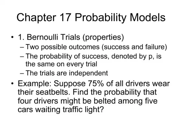
Chapter 17: Probability Models Last chapter in this unit!
Bernoulli Trials • Only 2 possible outcomes • Success / Failure • P for each success is constant • Trials independent [requiring n is infinite OR n < 10% population (10% Condition)] • Examples? • New notation: P(#trials = 1) = 0.20 P(#trials = 3) = (0.20)(0.80)(0.20) note #P = #trials
10% Condition makes sense? • It’s not intuitive to say that we MUST take a small n (10% of pop or less) to then model our pop. • However, this is a mathematical requirement (yes, proven; n/N needs to be tiny) • Finite population correction (fpc) fpc = Sqrt(1-(n/N)) • Standard Error = (std dev)/Sqrt(n) • approximation is exact if fpc is 1, or close to exact if close to 1 • You SHOULD ALWAYS find measures of error or variation and evaluate these; therein you can decide if your sample may not be representative of the pop. • Note our models ALWAYS include variation or std.dev.
Geometric Probability Model • How long will it take until I succeed? • Let p = success Let q = 1-p = failure • Let model = Geom(p) • Achieving first success on trial N requires first experiencing N-1 failures • P(#trials=N) = qN-1p • Expected value = μ = 1/p Std. Dev. = σ =SqRt(q/p2)
Example • People with O- blood are universal donors, but only exist as 6% of the population. If donors line up at random, how many do you expect to examine before you find a O- donor? What is the P that the first O- donor is one of the first four people in line? • p = success = O- q = failure = other blood type • Trials are not independent as n is finite, but donors are fewer than 10% of all possible donors. • Let X be number trials until find O- • Model is Geom(0.06) • E(X) = 1/0.06 = 16.7 Std Dev = Sqrt[0.94/(0.06)2]=16.16 • P(X<4) = P(X=1) + P(X=2) + P(X=3) + P(X=4) = (0.06) + (0.94)(0.06)+(0.94)(0.94)(0.06) + (0.94)3(0.06) = 0.2193 Blood drive expect to examine 16.7 people to find a O- donor. About 21.93% of the time, there will be one within the first four people in line.
TI for Geom P Model • 2nd DISTR • geometpdf() : probability density function • geometpdf(p, number of trials until success) • Try this with our last example: geometpdf(0.06, 4) • Gives P of any individual outcome • geometcdf(): cumulative density function • Sum of all P of several possible outcomes • geometcdf (p, number of trials) • Returns P of success on or before number of trials • geometcdf(0.06, 4) = P that O- donor found on or before 4th person.
Binomial Model • How many successes will I get after t time? • Was: P(#trials = 2)… Now: P(#successes = 2) Binomial Probability using Binomial Model (n, p) • Calculation includes p, q, and all combinations of outcomes • Orders of outcomes are disjoint • Use Addition Rule • Total number of combinations = “n Choose k” = (nk)= nCk = n!/(k!(n-k)!) where n! = n x (n-1) x (n-2) x … x 1 So Binomial Probability = P(#successes = x) = nCxpxqn-x Expected value = μ=npσ = Sqrt(npq)
Binomial vs. Geometric vs. Normal a) How many successes will I get after t time? b) How long will it take until I succeed? c) What is P of success for a range of times? • Which question (a, b, or c) is associated with each: Geometric, Binomial, or Normal Models. • Which model requires Bernoulli Trials? • Which involves discrete outcomes? Continuous outcomes?
Example Suppose 20 donors come to the blood drive. • What are mean and std dev of number of O- donors among them? • What is P that there are 2 or 3 O- donors? • Let p = O- donor = success = 0.06 • Let q = not O- donor = failure = 1 – 0.06 = 0.94 • Let X be number of O- among n=20 donors • Model X with Binom(20, 0.06) • E(X) = np = 20(0.06) = 1.2 • SD(X) = Sqrt(npq) = Sqrt(20(0.06)(0.94)) = 1.06 • P(X = 2 or 3) = P(X=2) + P(X=3) =(202)(0.06)2(0.94)18 + (203)(0.06)3(0.94)17 = 0.3106 In groups of 20 randomly selected donors, I expect to find an average of 1.2 universal donors with a std dev of 1.06. About 31% of the time, I’d find 2 or 3 O- donors in a set of 20 people.
TI Binomial Model 2nd DISTR binompdf(n, p, X) Probability Density Function (for Binomial Model) find P of individual outcome X = desired number of successes Try: binompdf(20, 0.06, 2) P that 2 O- donors in donor set of 20; get 0.2246 binomcdf(n, p, x) find P of getting x or fewer successes in n trials Cumulative Binomial Function Try: P of finding up to 10 O- donors in set of 20? binomcdf(20, 0.06, 10) Try: P of finding at least 10 O- donors in set of 20? (not <9) 1 - binomcdf(20, 0.06, 9)
Help for calculating huge values… or huge sets… For “large enough” n: Binomial Model (np, Sqrt(npq)) approximated by a Normal Model (np, Sqrt(npq)) So… You can calculate z, P just like for a Normal Model! What’s large enough? Success/Failure Condition: Binomial model is approx Normal if we expect at least 10* successes and 10* failures: np>10 and nq>10 * Technically 9, based on being w/in 3 std deviations, but this rule has been simplified (proof p. 395)
Continuous Random Variables • Caution! • Binomial Model = Discrete P for specific counts • Normal Model = Continuous P for any range of values • So… if you use an approximate Normal Model for a Binomial Model, there is no way to report the exact P for a specific value.