Download
1 / 27
280 likes | 506 Vues
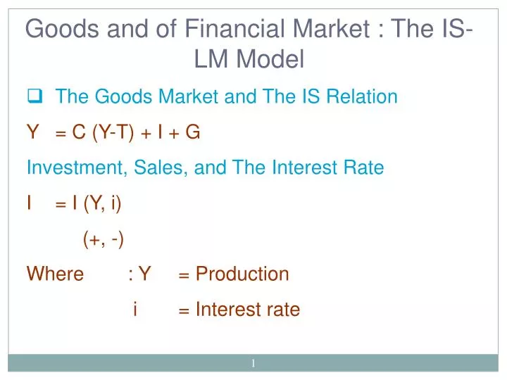
Goods and of Financial Market : The IS-LM Model. The Goods Market and The IS Relation Y = C (Y-T) + I + G Investment, Sales, and The Interest Rate I = I (Y, i) (+, -) Where : Y = Production i = Interest rate. The IS Curve Y = C (Y-T) + I (Y, i) + G

E N D
Goods and of Financial Market : The IS-LM Model • The Goods Market and The IS Relation • Y = C (Y-T) + I + G • Investment, Sales, and The Interest Rate • I = I (Y, i) • (+, -) • Where : Y = Production • i = Interest rate
The IS Curve Y = C (Y-T) + I (Y, i) + G The supply of goods (the left side) must be equal to the demand for goods (the right side)
The Effects of an Increase in The Interest rate on Output ZZ Demand, z For interest rate, i A ZZ’ For interest rate I’>i A’ Y’ Y Output, Y
The Derivation of the IS Curve ZZ ZZ’ A A’ Y’ Y Output, Y Interest rate, i A’ i’ A i IS curve Y’ Y Output, Y
The Shifts in the IS Curve Interest rate, i i IS ( For taxes T) IS ( for T’>T) Y Y’ Output, Y
Financial Markets and The LM Relation MS = M d M = $ YL (i) Variable M on The left side is the nominal money stock M/P = Y L (i) ………….. LM Relation
Interest rate, i A’ i’ A i M d (for Income Y) M/P Real Money, M/P) The effects of an increase in Income on the interest rate M d’ (for Y’> Y)
Interest rate, i Interest rate, i LM A’ A’ I’ I’ M d’ (for Y’> Y) A A i i M d (for Income Y) Y Y’ M/P (Real Money, M/P) The Derivation of The LM Curve Income, Y
LM (for M/P) Interest rate, i LM ‘ (for M’/P > M/P) i An Increase in Money i’ Y Income, Y Shifts in The LM Curve
The IS-LM Model : Exercises IS Relation Y = C(Y-T)+I(Y, i) + G LM Relation M/P = Y L( i )
Equilibrium in Financial Market (LM) i Income, Y Y The IS-LM Model Interest rate, i Equilibrium in Goods Market (IS)
Fiscal Policy, Activity, and The Interest Rates Decrease in G-T Fiscal contraction/ Fiscal Consolidation Increase in G-T Fiscal Expansion
In answering this or any question about the effects of Changes in policy, always follow these three steps : • Ask how this change affects good and financial market equilibrium relations , how its shifts the IS or/and the LM Curve • Characterize the effects of these shifts on the equilibrium • Describe the effects in the words
How The Increase in Taxes • The Increase in taxes affects equilibrium in the goods market (IS) • The increase in taxes affects decreases consumption ( because people have less disposable income ) and through the multiplier, decreases output • What Happens to the LM Curve ? nothing
Interest rate, i LM i i’ IS (for T) IS’ (for T’> T) Y’ Y Output, Y The effects of an Increase in Taxes An Increase in taxes shifts the IS curve to the left, and leads to a decrease in equilibrium output and the equilibrium interest rate
Monetary Policy, Activity, and The Interest Rates Increase in Money (M) Monetary expansion Decrease in Money (M) Monetary Contraction/ Monetary Tightening
How The Central Bank Increases Nominal Money, through open market operation (Price level is fixed) • The Increase in Nominal money affects equilibrium in the Financial market (LM) • An increase in money shifts the LM down • What Happens to the IS Curve ? Nothing
Interest rate, i LM (for M/P) LM’ (for M’/P) > M/P) A monetary expansion leads to higher output and a lower interest rate i I’ IS Y Y’ Output, Y The effects of a monetary Expansion
Using a Policy Mix • Some times monetary and fiscal policies is used to offset the adverse on the demand for goods of fiscal contraction • Some times the monetary-fiscal mix emerges from tensions or even disagreements between the government (which is in charge of fiscal policy) and the central bank (which is in charge of monetary policy)
LM Interest rate, i LM’ The Right Combination of deficit reduction and monetary expansion can achieve a reduction in the deficit without adverse effects on output A i B IS A’ I’ IS’ Y Output, Y Deficit Reduction and Monetary Expansion
Adding Dynamics • Source of dynamics in goods market : • Production adjusts slowly to demand • Demand (consumption and investment) adjusts slowly to income (production) • Slow adjustment of Y in goods market • Fast adjustment of i in financial market
Goods Market Financial Market Interest rate, i LM’ LM Output decreases slowly Interest rate Adjust Instantaneously iB B B A iA IS iA A IS’ YB YA YA Output, Y Output, Y Output Increases slowly Interest rate, i
Interest rate, i LM’ LM A’’ i’’ A’ i’ A i IS Y’ Y The Dynamic effects of a Monetary contraction A monetary contraction leads To an increase in the interest Rate. The Increase in the Interest rate leads, over time To decline in output Output, Y
Monetary and Fiscal Policy : an Example Consider the following IS-LM Model : C = 200 + 0.25 YD I = 150 + 0.25 Y – 1000 I G = 250 T = 200 (M/P) d = 2Y- 8000 i M/P = 1,600
Derive the equation for the IS curve • Derive the equation for LM curve • Solve for equilibrium real output • Solve equilibrium interest rate • Solve for equilibrium values of C and I • Now Suppose that the money supply increases to M/P = 1840. Solve Y, i, C and explain in words the effects of expansionary monetary policy • Set M/P equal its initial value of 1600, Now suppose that government spending increase to G = 400. Summarize the effects of expansionary fiscal policy on Y, i and C. and why if government spending decrease to G = 100