Download
1 / 25
250 likes | 414 Vues
Outdoor SLAM using Visual Appearance and Laser Ranging P. Newman, D. Cole and K. Ho ICRA 2006. Jackie Libby Advisor: George Kantor. Main Idea. laser and camera for 3d SLAM system Laser: builds 3d point cloud map Camera: detects loop closure from sequences of images

E N D
Outdoor SLAM using Visual Appearance and Laser RangingP. Newman, D. Cole and K. HoICRA 2006 Jackie Libby Advisor: George Kantor
Main Idea • laser and camera for 3d SLAMsystem • Laser: builds 3d point cloud map • Camera: detects loop closure from sequences of images • First working implementation in outdoor environment
Outline • Slam framework • Laser data representation • How loop is detected with vision • How loop is closed once detected • results
SLAM representation: state x(k+1|k) = state vector of vehicle poses from t = 1, …, k+1 given observations from t = 1, …, k xvn = nth vehicle pose in state vector u(k+1) = odometry between k and k+1 = SΕ3 transformation composition operator (motion model)
SLAM representation: covariance Pv = covariance of newly added vehicle state (bottom left) Pvp = ? (my guess: covariance between new state and all previous states)
Scan-match framework • Nodding “yes-yes” laser • Returns planar scans at different elevations • each vehicle pose corresponds to a laser scan • xv(k) -> Sk • timesteps not constant • xv(i), xv(j) -> Si, Sj -> Ti,j • Ti,j = rigid transformation • Observation -> EKF equations • i, j sequential -> Ti,j can replace u • loop closing -> j >> i • Ti,j used to correct position
State vector with growing uncertainty • outdoor data set • x,y,z grid (20m marks) • 1 σ x,y,z uncertainty ellipsoids • Effect of long loops • How to detect loop closure • slam pdf, small Mahalanobis distance • - Ellipsoids overconfident -> this method fails • Vision system • - Matches image sequences • - similarity in appearance
My work with SLAM: • CASC • Advisor: George Kantor • Sanjiv Singh • Marcel Bergerman • Ben Grocholsky • Brad Hamner • Retroreflectivecones • no-no nodding SICK laser
Detecting loop closure (high level) • Assumption: • 2 images look similar -> close in space • Not close in time -> loop detected • Problem: • Just one image pair -> false positive • “repetitious low level descriptors” • “common texture” • leaves, bricks on buildings • “background similarity” • “common large scale features” • plants, windows • Solution: • sequences of image pairs increases confidence
Image, Iu • Detect interest points • Harris Affine detector • Scale invariant, affine invariant • Example: corners -> still a corner from any angle or scale Thanks Martial Hebert!
Detect interest points (ignore blue circles) SIFT Descriptors {d1, …, dn} • 16x16 pixel window around interest point • Assign each pixel a gradient orientation (out of 8 values) • For each 4x4 window, make histogram of orientations • 16 histograms * 8 values = 128 = dimension of SIFT vector Thanks Martial Hebert!
SIFT Descriptors {d1, …, dn} • Clustered into words, • Vocab = set of all words • SIFT Descriptors: n is different for different images • word, = {d1, …, dk} • clustering happens in an offline learning process • Vocabulary, V • future work: different vocabularies for different settings • urban, park, indoors
The more frequent the word, the less descriptive it is • inverse weighting frequency scheme *: • Vocab = set of all words • weight for each word wi = weight for index word, N = total # images ni = # images where this word appears *K. S. Jones, “Exhaustivity and specificity,” Journal of Documentation, vol. 28, no. 1, pp. 11–21, 1972.
weight for each word • Image vector of weights • Image has been transformed into a vector • vector is long, |V|, but many elements are zero
Image • Image Cosine distance: cos(0) = 1 The closer the vectors -> the smaller the angle between them the greater the similarity • Similarity
Similarity Matrix • Similarity matrix, M • Mi,j = S(i,j) • darker means more similar • axes = timesteps • same for x and y • comparing each image against every other one • main diagonal is line of reflection • Loop closure = off diagonal streaks • ai bi • ai+1 bi+1 • Boxes = false positives • one to many mapping: • ai bi+1, bi+2, bi+3 … • bi ai+1, ai+2, ai+3 … • causes: • vehicle stopped • repetitive low-level structure (windows, bricks, leaves) • distant images
Sequence extraction (finding streaks) Maximal cumulative similarity • Modified Smith-Waterman algorithm • dynamic programming • penalty terms avoid boxes • allow for curved lines (i.e. change in velocity) • α term allows gaps • Maximum Hi,j = ηA,B
Removing “common mode similarity” (finding boxes) Decompose M into sum of outer products “Dominant structure” = repetitive structure dominant structure largest eigenvalues/vectors First three outer products Eigenface: More repetition -> more range in eigenvalues Relative significance: Maximize entropy:
Sequence Significance • problem: • Maximum Hi,j = ηA,B this doesn’t mean there’s a loop • solution: • randomly shuffle rows and columns of M, recompute ηA,B • look at distribution: Extreme value distribution (EVD) Probability that sequence could be random ηA,B = real score η = random score threshold at 0.5%
Estimating Loop Closure Geometry • We have detected a loop (with image sequence) • Now how do we close it? (how do we find Tij?) • One solution: iterative scan matching • ηA,B ai, bj xvi , xvj Si, Sj Tij • Problem: local minima • Better solution: projective model • Essential matrix • 5 point algorithm with Ransac loop • User lasers to: • Remove scale ambiguity • Fine-tune with iterative scan matching • quality of final scan match is another quality check
Enforcing loop closure • Naïve method: single EKF update step • only works for small errors, because of linear approximation • Better method: • constrained non-linear optimization • incremental changes [xv1, …., xvn] [T1,2, … Tn-1,n, Tn,1] [Σ1,2, …, Σn,1] (from scan-matching) Want new poses, [T*1,2, … T*n-1,n, T*n,1] Minimize: Subject to constraint:
Results Resulting estimated map And vehicle trajectory • successfully applied to several data sets • 98% runtime spent on laser registration -> bottleneck • 1/3 real time • most expensive part of vision subsystem is feature detector/descriptor • (Harris Affine/ SIFT)
Conclusions and future work • Conclusions • SLAM system for outdoor applications • Works for challenging urban environment • Complementary vision laser system • Vision for loop closing • Laser data for geometry map building • First working implementation • Future work • SLAM formulation not efficient • Laser scan matching is bottle neck • Learning vocabularies for distinct domains • (urban, park, indoors) • Different similarity matrix if domain switches