Testing Scenarios for Characterizing Process Equivalences in Probabilistic Automata
This paper discusses various process equivalences, including bisimulation and ready trace, and evaluates their justification through testing scenarios—particularly focusing on probabilistic automata. We define testing scenarios and observe the limitations of distinguishing processes through observation. The results relate to developing a statistical hypothesis testing framework to assess the equivalence based on outcomes observed when interacting with probabilistic systems. The implications of these findings are critical for advancing concurrency theory and understanding process behavior.

Testing Scenarios for Characterizing Process Equivalences in Probabilistic Automata
E N D
Presentation Transcript
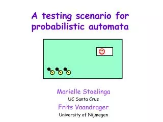
A testing scenario for probabilistic automata Marielle Stoelinga UC Santa Cruz Frits Vaandrager University of Nijmegen
?? ´ P Q Characterization of process equivalences • process equivalences • bisimulation / ready trace / ... equivalence • algebraical / logical / denotional / ... definitions • are these reasonable ? • justify equivalence via testing scenarios / button pushing experiments • comparative concurrency theory • De Nicola & Hennesy [DH86], Milner [Mil80], van Glabbeek [vGl01] • testing scenarios: • define intuitive notion of observation, fundamental • processes that cannot be distinguished by observation ce ´:P ´ Q iff Obs(P) = Obs(Q) • ´ does not distinguish too much/too little
?? ´ P Q Characterization of process equivalences • process equivalences • bisimulation / ready trace / ... equivalence • algebraical / logical / denotional / ... definitions • are these reasonable ? • justify equivalence via testing scenarios / button pushing experiments • testing scenarios: • define intuitive notion of observation, fundamental • processes that cannot be distinguished by observation are deemed to be equivalent • justify process equivalence ´:P ´ Q iff Obs(P) = Obs(Q) • ´ does not distinguish too much/too little
Main results • testing scenarios in non-probabilistic case • trace equivalence • bisimulation • ... • we define • observations of a probabilistic automaton (PA) • observe probabilities through statistical methods (hypothesis testing) • characterization result • Obs(P) = Obs(Q) iff trd(P) = trd(Q), P, Q finitely branching • trd(P) extension of traces for PAs. [Segala] • justifies trace distr equivalence in terms of observations
Model for testing scenarios display a machine buttons • machine M • a black box • inside: process described by LTS P • display • showing current action • buttons • for user interaction
Model for testing scenarios display a machine buttons • an observer • records what s/he sees (over time) + buttons • define ObsM(P): • observations of P = what observer records, if LTS P is inside M
a Trace Machine (TM) • no buttons for interaction • display shows current action
P a a b c Trace Machine (TM) • no buttons for interaction • display shows current action • with P inside M, an observer sees one of e, a, ab, ac • ObsTM(P) = traces of P • testing scenario justifies trace (language) equivalence
a Trace Machine (TM) • no distinguishing observation between a a a b c b c
d reset Trace Distribution Machine (TDM) P h t 1/2 1/2 d l • reset button: start over • repeat experiments • each experiment yields trace of same length k (wlog) • observefrequencies of traces
d reset Trace Distribution Machine (TDM) P h t 1/2 1/2 d l • 100 exps, length 2frequencies - hd tl tl hd tl .... hd hd 48 tl52 other 0 (hh,dh,hl,...)
d reset Trace Distribution Machine (TDM) P h t 1/2 1/2 d l not every seq of experiments is an observation • with many experiments: #hd¼ # tl • 100 exps, length 2frequencies - hd tl tl hd tl .... hd hd 48 tl52 other 0
d reset Trace Distribution Machine (TDM) P h t 1/2 1/2 d l • with many experiments: #hd¼ # tl • 100 exps, length 2frequencies - hd tl tl hd tl ... hd hd 48 tl52 other 0 - hd hd hd hd .... hd hd 100 tl 0 other 0 2 Obs(P) freq likely 2 Obs(P) freq unlikely /
d reset Trace Distribution Machine (TDM) P d b c b 3/4 1/3 2/3 1/4 • nondeterministic choice • choose one transition probabilistically • in large outcomes: 1/2 #c + 1/3 #d ¼ #b • use statistics: • b,b,b,....b2 Obs(P) freqs likely • b,d,c,b,b,b,c,...2 Obs(P) freqs unlikey /
a reset Observations TDM P h t 1/2 1/2 d l • ObsTDM(P) = { s | s is likely to be produced by P}
a reset Observations TDM P h t 1/2 1/2 d l • perform m experiments (m resets) • each experiment yields trace of length k(wlog) • sequence s2 (Actk)m • Obs(P) = {s2 (Actk)m | s is likely to be produced by P, k,m 2N} • what is likely? use hypothesis testing
h t 1/2 1/2 Which frequencies are likely? • I have a sequence s = h,t,t,t,h,t,...2 {h,t}100 • I claim: generated s with automaton P. • do you believe me • if s contains 15 h’s? • if s contains 42 h’s?
h t 1/2 1/2 0 40 50 60 100 reject H0 K: accept H0 reject H0 Which frequencies are likely? • I have a sequence s = h,t,t,t,h,t,...2 {h,t}100 • I claim: generated s with automaton P. • do you believe me • if s contains 15 h’s? • if s contains 42 h’s? • use hypothesis testing: • fix confidence level a 2 (0,1) • H0 null hypothesis = s is generated by P #h
h t 1/2 1/2 0 40 50 60 100 reject H0 K: accept H0 reject H0 Which frequencies are likely? • I have a sequence s = h,t,t,t,h,t,...2 {h,t}100 • I claim: generated s with automaton P. • do you believe me • if s contains 15 h’s? • if s contains 42 h’s? • use hypothesis testing: • fix confidence level a 2 (0,1) • H0 null hypothesis = s is generated by P • PH0[K] > 1-a: prob on false rejection ·a P: H0[K] minimal : prob on false acceptance minimal #h
h t 1/2 1/2 0 40 50 60 100 reject H0 K: accept H0 reject H0 Which frequencies are likely? • I have a sequence s = h,t,t,t,h,t,...2 {h,t}100 • I claim: generated s with automaton P. • do you believe me • if s contains 15 h’s? NO • if s contains 42 h’s? YES • use hypothesis testing: • fix confidence level a 2 (0,1) • H0 null hypothesis = s is generated by P • PH0[K] > 1-a: prob on false rejection ·a P: H0[K] minimal : prob on false acceptance minimal #h
h t 1/2 1/2 Example: Observations for a =0.05 • Obs(P) = {s2 (Actk)m | s is likely to be produced by P, k,m2N } • for k = 1 and m = 100 s2 (Act)100 is an observation iff 40 · freqs (hd) · 60 60 50 40 0 100 K1,100
h t 1/2 1/2 Example: Observations for a =0.05 • Obs(P) = {s2 (Actk)m | s is likely to be produced by P, k,m2N } • for k = 1 and m = 100 s2 (Act)100 is an observation iff 40 · freqs (hd) · 60 • for k = 1 and m = 200 s2 (Act)200 is an observation iff 88 · freqs (h) · 112 • etc .... 112 100 88 0 200 K1,200
h t 1/2 1/2 Example: Observations for a =0.05 • Obs(P) = {s2 (Actk)m | s is likely to be produced by P, k,m2N } • for k = 1 and m = 100, s2 (Act)100 is an observation iff 40 · freqs (hd) · 60 • for k = 1 and m = 200 s2 (Act)200 is an observation iff 88 · freqs (h) · 112 • etc .... exp freq EP alloweddeviation e ( = 12) 112 100 88 0 0 200 K1,200
With nondeterminism P a c b a 3/4 1/3 2/3 1/4 • s = b,c,c,d,b,d,....,c2 Obs(P) ??
With nondeterminism P a c b a 3/4 1/3 2/3 1/4 • s = b,c,c,d,b,d,....,c2 Obs(P) ?? • fix schedulers: p1, p2, p3... p100 • pi = P[take left trans in experiment i] • 1 - pi = P[takerighttrans in experiment i] • H0: s is generated by P under p1, p2, p3... p100 • critical section Kp1,...,p100
With nondeterminism P a c b a 3/4 1/3 2/3 1/4 • s = b,c,c,d,b,d,....,c2 Obs(P) ?? • fix schedulers: p1, p2, p3... p100 • pi = P[take left trans in experiment i] • 1 - pi = P[takerighttrans in experiment i] • H0: s is generated by P under p1, p2, p3... p100 • critical sectionKp1,...,p100 s2 Obs(P) iff s2Kp1,...,p100 for some p1, p2, p3... p100
Example: Observations b d c b 3/4 1/3 2/3 1/4 Observations for k =1, m = 100. • s contains b,c only with 54 · freqs (c) · 78 • take pi = 1 for all i • s contains b,d only with 62 · freqs (d) · 88 • take pi = 0 for all i
Example: Observations b d c b 3/4 1/3 2/3 1/4 Observations for k =1, m = 100. • s contains a,b only and 54 · freqs (c) · 78 • take pi = 1 for all i • s contains b,d only and 62 · freqs (d) · 88 • take pi = 0 for all i Observations for k=1, m = 200 • 61 · freqs (c) · 71 and 70 · freqs (d) · 80 • pi = ½ for all i (exp 66 c’s; 74 d’s; 60 b’s) • (these are not all observations; they form a sphere)
Main result • TDM characterizes trace distr equivalence ObsTDM(P) = ObsTDM(Q)ifftrd(P) = trd(Q) if P, Q are finitely branching • justifies trace distribution equivalence in an observational way
Main result TDM characterizes trace distr equiv ´TD ObsTDM(P) = ObsTDM(Q) iff trd(P) = trd(Q) • “only if” part is immediate, “if”-part is hard. • find a distinguishing observation if P, Q have different trace distributions. • IAP for P. Q fin branching • P, Q have the same infinite trace distrs iff P, Q have the same finite trace distrs • the set of trace distrs is a polyhedron • Law of large numbers • for random vars with different distributions
h t 1/2 1/2 0 40 50 60 100 K Observations a =0.05 • Obs(P) = {s2 (Actk)m | s likely to be produced by P} • Obs(P) = {s2 (Actk)m | freq_s in K} • for k = 1 and m = 100, b2 (Act)100 is an observation iff 40 · freqb (hd) · 60
h t 1/2 1/2 Nondeterministic case • \sigma = \beta_1 ,...\beta_m • fixed adversaries • take in • expect_freq • for \gamma\in Act^k, freq_\gamma(\beta) freq \in \ • we consider only frequency of traces in an outcome
a! a b c b! a? b?
a! b! a?
d reset Trace Distribution Machine (TDM) h t 1/2 1/2 d l • reset button: start over • repeat experiments: yields sequenceof traces • in large outcomes: #hd¼ # tl • use statistics: • hd,hd,hd,...,hd2 Obs(P) too unlikely • hd,tl,tl,hd,...tl,hd2 Obs(P) likely /
h t 1/2 1/2 0 40 50 60 100 exp freq
Testing scenario’s display a machine buttons • a black box with display and buttons • inside: process described by LTS P • display: current action • what do we see (over time)? ObsM(P) • P, Q are deemed equivalent iff ObsM(Q) = ObsM(Q) • desired characterization:
h t 1/3 1/3 Observations a =0.05 • Obs(P) = {s2 (Actk)m | s is likely to be produced by P} • for k = 1 and m = 99, • expectation E = (33,33,33) • Obs(P) = {s2 (Act)99 | | s – E | < 15}