2. Comparing biological sequences : sequence alignment
2. Comparing biological sequences : sequence alignment. DNA Sequence Comparison: First Success Story. Finding sequence similarities with genes of known function is a common approach to infer a newly sequenced gene’s function

2. Comparing biological sequences : sequence alignment
E N D
Presentation Transcript
DNA Sequence Comparison: First Success Story • Finding sequence similarities with genes of known function is a common approach to infer a newly sequenced gene’s function • In 1984 Russell Doolittle and colleagues found similarities between cancer-causing gene (v-sys in Simian Sarcoma Virus) and normal growth factor (PDGF) gene
So what? • Identifying the similarity between PDGF and the viral oncogene helped lead to a modern hypothesis of cancer. • Identifying the similarity between ATP binding ion channels and the Cystic Fibrosis gene led to a modern hypothesis of CF. • Comparing sequences can yield biological insight. 3
Similarity • Similar genes may have similar functions • Similar genes may have similar evolutionary origins • Similarity between sequences is not a vague idea---it can be quantified • But...how do we compute it?
Complete DNA Sequences nearly 200 complete genomes have been sequenced
Evolution at the DNA level Deletion Mutation …ACGGTGCAGTTACCA… SEQUENCE EDITS …AC----CAGTCCACCA… REARRANGEMENTS Inversion Translocation Duplication
Evolutionary Rates next generation OK OK OK X X Still OK?
Sequence conservation implies function • Alignment is the key to • Finding important regions • Determining function • Uncovering the evolutionary forces
Sequence Alignment AGGCTATCACCTGACCTCCAGGCCGATGCCC TAGCTATCACGACCGCGGTCGATTTGCCCGAC -AGGCTATCACCTGACCTCCAGGCCGA--TGCCC--- TAG-CTATCAC--GACCGC--GGTCGATTTGCCCGAC Definition Given two strings x = x1x2...xM, y = y1y2…yN, an alignment is an assignment of gaps to positions 0,…, N in x, and 0,…, N in y, so as to line up each letter in one sequence with either a letter, or a gap in the other sequence
Apologia for a diversion... • Computing similarity is detail-oriented, and we need to do some preliminary work first: • The Manhattan Tourist Problem introduces grids, graphs and edit graphs 11
Manhattan Tourist Problem Where to? See the most stuff in the least time.
Manhattan Tourist Problem (MTP) Imagine seeking a path (from source to sink) to travel (only eastward and southward) with the most number of attractions (*) in the Manhattan grid Source * * * * * * * * * * * Sink
Manhattan Tourist Problem: Formulation Goal: Find the longest path in a weighted grid. Input: A weighted grid G with two distinct vertices, one labeled “source” and the other labeled “sink” Output: A longest path in G from “source” to “sink”
19 13 15 20 23 0 9 5 3 MTP: An Example 0 1 2 3 4 j coordinates source 3 2 4 0 0 1 0 4 3 2 2 3 2 4 1 1 6 5 4 2 0 7 3 4 2 i coordinates 4 5 2 4 1 0 2 3 3 3 3 8 5 6 5 2 sink 1 3 2 4
13 32 19 15 34 30 10 17 22 20 9 4 1 3 0 5 MTP: An Example 0 1 2 3 4 j coordinates source 3 2 4 0 0 1 0 4 3 2 2 3 2 4 1 1 6 5 4 2 0 7 3 4 2 i coordinates 4 5 2 4 1 0 2 3 3 3 3 8 5 6 5 2 sink 1 3 2 4
MT(n,m) x MT(n-1,m)+ length of the edge from (n- 1,m) to (n,m) y MT(n,m-1)+ length of the edge from (n,m-1) to (n,m) return max{x,y} MTP: Simple Recursive Program
MT(n,m) x MT(n-1,m)+ length of the edge from (n- 1,m) to (n,m) y MT(n,m-1)+ length of the edge from (n,m-1) to (n,m) return max{x,y} Slow, for the same reason that RecursiveChange was slow MTP: Simple Recursive Program
MTP: Dynamic Programming j 0 1 source 1 0 1 S0,1 = 1 i 5 1 5 S1,0 = 5 • Instead of recursion, store the result in an array S
MTP: Dynamic Programming j 0 1 2 source 1 2 0 1 3 S0,2 = 3 i 5 3 -5 1 5 4 S1,1 = 4 3 2 8 S2,0 = 8
MTP: Dynamic Programming j 0 1 2 3 source 1 2 5 0 1 3 8 S3,0 = 8 i 5 3 10 -5 1 1 5 4 13 S1,2 = 13 5 3 -5 2 8 9 S2,1 = 9 0 3 8 S3,0 = 8
MTP: Dynamic Programming j 0 1 2 3 source 1 2 5 0 1 3 8 i 5 3 10 -5 -5 1 -5 1 5 4 13 8 S1,3 = 8 5 3 -3 3 -5 2 8 9 12 S2,2 = 12 0 0 0 3 8 9 S3,1 = 9
MTP: Dynamic Programming (cont’d) j 0 1 2 3 source 1 2 5 0 1 3 8 i 5 3 10 -5 -5 1 -5 1 5 4 13 8 5 3 -3 2 3 3 -5 2 8 9 12 15 S2,3 = 15 0 0 -5 0 0 3 8 9 9 S3,2 = 9
MTP: Dynamic Programming (cont’d) j 0 1 2 3 source 1 2 5 0 1 3 8 Done! i 5 3 10 -5 -5 1 -5 1 5 4 13 8 (showing all back-traces) 5 3 -3 2 3 3 -5 2 8 9 12 15 0 0 -5 1 0 0 0 3 8 9 9 16 S3,3 = 16
si-1, j + weight of the edge between (i-1, j) and (i, j) si, j-1 + weight of the edge between (i, j-1) and (i, j) max si, j = MTP: Recurrence Computing the score for a point (i,j) by the recurrence relation: the running time is n x m for a n by m grid (n = # of rows, m = # of columns)
A2 A3 sA1 + weight of the edge (A1, B) sA2 + weight of the edge (A2, B) sA3 + weight of the edge (A3, B) max of sB = A1 B Manhattan Is Not A Perfect Grid What about diagonals? • The score at point B is given by:
max of sy + weight of vertex (y, x) where y є Predecessors(x) sx = Manhattan Is Not A Perfect Grid (cont’d) Computing the score for point x is given by the recurrence relation: • Predecessors (x) – set of vertices that have edges leading to x • The running time for a graph G(V, E) (V is the set of all vertices and E is the set of all edges) is O(E) since each edge is evaluated once
Traversing the Manhattan Grid a) b) • 3 different strategies: • a) Column by column • b) Row by row • c) Along diagonals c)
Aligning DNA Sequences n = 8 V = ATCTGATG matches mismatches insertions deletions 4 m = 7 1 W = TGCATAC 2 match 3 mismatch V W deletion indels insertion
Longest Common Subsequence (LCS) Problem • Given two sequences • v = v1 v2…vm and w = w1 w2…wn • The LCS of v and w is a sequence of positions in • v: 1 < i1 < i2 < … < it< m • and a sequence of positions in • w: 1 < j1 < j2 < … < jt< n • such that it -th letter of v equals to jt-letter of w and t is maximal
0 8 1 7 6 2 5 2 4 3 3 1 5 0 7 6 5 3 2 0 4 6 LCS: Example i coords: elements of v A T -- C -- T G A T G elements of w -- T G C A T -- A -- C j coords: (0,0) (1,0) (2,1) (2,2) (3,3) (3,4) (4,5) (5,5) (6,6) (7,6) (8,7) positions in v: 2 < 3 < 4 < 6 Matches shown inred positions in w: 1 < 3 < 5 < 6 The LCS Problem can be expressed using the grid similar to Manhattan Tourist Problem grid…
LCS: Dynamic Programming • Find the LCS of two strings Input: A weighted graph G with two distinct vertices, one labeled “source” one labeled “sink” Output: A longest path in G from “source” to “sink” • Solve using an LCS edit graph with diagonals replaced with +1 edges
LCS Problem as Manhattan Tourist Problem A T C T G A T C j 0 1 2 3 4 5 6 7 8 i 0 T 1 G 2 C 3 A 4 T 5 A 6 C 7
Edit Graph for LCS Problem A T C T G A T C j 0 1 2 3 4 5 6 7 8 i 0 T 1 G 2 C 3 A 4 T 5 A 6 C 7
si-1, j si, j-1 si-1, j-1 + 1 if vi = wj max si, j = Computing LCS Let vi = prefix of v of length i: v1 … vi and wj = prefix of w of length j: w1 … wj The length of LCS(vi,wj) is computed by:
Computing LCS (cont’d) i-1,j i-1,j -1 0 1 si-1,j + 0 0 i,j -1 si,j = MAX si,j -1 + 0 i,j si-1,j -1 + 1, if vi = wj
4 2 3 6 6 6 5 4 3 1 3 2 1 3 5 6 LCS Problem Revisited V = ATCTGATG = V1, V2, …, Vn where n = 8 W = TGCATAC = W1, W2, …, Wm where m = 7 i 1 , i 2 , i 3 , i 4 i < < < V j 1 , j 2 , j 3 , j 4 W < < < j i 1 ,j 1 i 1 ,j 1 i 2 ,j 2 Manhattan Tourist Problem is also the example of maximizing problem . i 2 ,j 2 . i 3 ,j 3 . i t ,j t
Alignment Grid Example W A T C G 0 1 2 2 3 4 V = A T - G T | | | W= A T C G – 0 1 2 3 4 4 V A T G T
A T T A A T A T T A T A A T T A Aligning Sequences without Insertions and Deletions: Hamming Distance Given two DNA sequences V and W : V : W : • The Hamming distance: dH(V, W) = 8 is large but the sequences are very similar
T A T A A T T A A T A T T A T A Aligning Sequences with Insertions and Deletions However, by shifting one sequence over one position: V : -- W : -- • The edit distance: dH(v, w) = 2. • Using Hamming distance neglects insertions and deletions in DNA
Edit Distance Levenshtein (1966) introduced edit distance of two strings as the minimum number of elementary operations (insertions, deletions, and substitutions) to transform one string into the other d(v,w) = MIN no. of elementary operations to transform vw
Edit Distance (cont’d) ith letter of v compare with ith letter of w V = - ATATATAT V = ATATATAT Just one shift Make it all line up W= TATATATA W = TATATATA Edit distance: d(v, w) = 2 (one insertion and one deletion)
Edit Distance: Example • 5 edit operations: TGCATAT ATCCGAT • TGCATAT (delete last T) • TGCATA (delete last A) • TGCAT (insert A at front) • ATGCAT (substitute C for 3rdG) • ATCCAT (insert G before last A) • ATCCGAT (Done)
Edit Distance: Example (cont’d) 4 edit operations: TGCATAT ATCCGAT TGCATAT (insert A at front) ATGCATAT (delete 6thT) ATGCATA (substitute G for 5thA) ATGCGTA (substitute C for 3rdG) ATCCGAT (Done)
T A G T C C A T T G A A T Alignment: 2 row representation Given 2 DNA sequences v and w: v : m = 7 w : n = 6 Alignment : 2 * k matrix ( k > m, n ) letters of v A T -- G T T A T -- letters of w A T C G T -- A -- C 4 matches 2 insertions 2 deletions
The Alignment Grid • 2 sequences used for grid • V = ATGTTAT • W = ATCGTAC • Every alignment path is from source to sink
A T C G T A C w 1 2 3 4 5 6 7 0 0 v A 1 T 2 G 3 T 4 T 5 A 6 T 7 Alignment as a Path in the Edit Graph 0 1 2 2 3 4 5 6 7 7 A T _ G T T A T _ A T C G T _ A _ C 0 1 2 3 4 5 5 6 6 7 (0,0) , (1,1) , (2,2), (2,3), (3,4), (4,5), (5,5), (6,6), (7,6), (7,7) - Corresponding path -
A T C G T A C w 1 2 3 4 5 6 7 0 0 v A 1 T 2 G 3 T 4 T 5 A 6 T 7 Alignments in Edit Graph (cont’d) • and represent indels in v and w with score 0. • represent matches with score 1. • The score of the alignment path is 5.
A T C G T A C w 1 2 3 4 5 6 7 0 0 v A 1 T 2 G 3 T 4 T 5 A 6 T 7 Alignment as a Path in the Edit Graph Every path in the edit graph corresponds to an alignment: