Population Dynamics
Population Dynamics. Focus on births (B) & deaths (D) B = bN t , where b = per capita rate (births per individual per time) D = dN t. N = bN t – dN t = (b-d)N t. Exponential Growth. Density-independent growth models Discrete birth intervals (Birth Pulse) vs.

Population Dynamics
E N D
Presentation Transcript
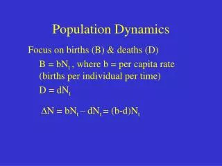
Population Dynamics • Focus on births (B) & deaths (D) • B = bNt , where b = per capita rate (births per individual per time) • D = dNt • N = bNt – dNt = (b-d)Nt
Exponential Growth • Density-independent growth models • Discrete birth intervals (Birth Pulse) • vs. • Continuous breeding (Birth Flow)
> 1 • < 1 • = 1 Nt = N0 t
Geometric Growth • When generations do not overlap, growth can be modeled geometrically. Nt = Noλt • Nt = Number of individuals at time t. • No = Initial number of individuals. • λ = Geometric rate of increase. • t = Number of time intervals or generations.
Exponential Growth • Birth Pulse Population (Geometric Growth) • e.g., woodchucks • (10 individuals to 20 indivuals) • N0 = 10, N1 = 20 • N1 = N0 , • where = growth multiplier = finite rate of increase > 1 < 1 = 1
Exponential Growth • Birth Pulse Population • N2 = 40 = N1 • N2 = (N0 ) = N0 2 • Nt = N0 t • Nt+1 = Nt
Exponential Growth • Density-independent growth models • Discrete birth intervals (Birth Pulse) • vs. • Continuous breeding (Birth Flow)
Exponential Growth • Continuous population growth in an unlimited environment can be modeled exponentially. dN / dt = rN • Appropriate for populations with overlapping generations. • As population size (N) increases, rate of population increase (dN/dt) gets larger.
Exponential Growth • For an exponentially growing population, size at any time can be calculated as: Nt = Noert • Nt = Number individuals at time t. • N0 = Initial number of individuals. • e = Base of natural logarithms =2.718281828459 • r = Per capita rate of increase. • t = Number of time intervals.
Nt = N0ert Difference Eqn Note: λ = er
Exponential growth and change over time N = N0ert dN/dt = rN Number (N) Slope (dN/dt) Time (t) Number (N) Slope = (change in N) / (change in time) = dN / dt
ON THE MEANING OF r • rm - intrinsic rate of increase – unlimited • resourses • rmax– absolute maximal rm • - also called rc = observed r > 0 r < 0 r = 0
Intrinsic Rates of Increase • On average, small organisms have higher rates of per capita increase and more variable populations than large organisms.
Growth of a Whale Population • Pacific gray whale (Eschrichtius robustus) divided into Western and Eastern Pacific subpopulations. • Rice and Wolman estimated average annual mortality rate of 0.089 and calculated annual birth rate of 0.13.
Growth of a Whale Population • Reilly et.al. used annual migration counts from 1967-1980 to obtain 2.5% growth rate. • Thus from 1967-1980, pattern of growth in California gray whale population fit the exponential model: Nt = Noe0.025t
Logistic Population Growth • As resources are depleted, population growth rate slows and eventually stops • Sigmoid (S-shaped) population growth curve • Carrying capacity (K):
Logistic Population Growth dN / dt = rN dN/dt = rN(1-N/K) • r = per capita rate of increase • When N nears K, the right side of the equation nears zero • As population size increases, logistic growth rate becomes a small fraction of growth rate
Limits to Population Growth • Environment limits population growth by altering birth and death rates • Density-dependent factors • Density-independent factors
Readings • 8.3 through 8.13; pp. 162-177 • Field Studies, pp. 164-165 • Ecological Issues, p. 175 • Ecological Issues, p. 219 • Field Studies, pp. 230-231
Logistic Population Model Nt = 2, R = 0.15, K = 450 A. Discrete equation - Built in time lag = 1 - Nt+1 depends on Nt
I. Logistic Population Model B. Density Dependence
Logistic Population ModelC. Assumptions • No immigration or emigration • No age or stage structure to influence births and deaths • No genetic structure to influence births and deaths • No time lags in continuous model
K Logistic Population ModelC. Assumptions • Linear relationship of per capita growth rate and population size (linear DD)
Logistic Population ModelC. Assumptions • Linear relationship of per capita growth rate and population size (linear DD)
I. Logistic Population Model Discrete equation Nt = 2, r = 1.9, K = 450 Damped Oscillations r <2.0
I. Logistic Population Model Discrete equation Nt = 2, r = 2.5, K = 450 Stable Limit Cycles 2.0 < r < 2.57 * K = midpoint
I. Logistic Population Model Discrete equation Nt = 2, r = 2.9, K = 450 • Chaos • r > 2.57 • Not random • change • Due to DD • feedback and time • lag in model
Underpopulation or Allee Effect b=d b=d d Vital rate b b<d r<0 N* K N
Review of Logistic Population ModelD. Deterministic vs. Stochastic Models Nt = 1, r = 2, K = 100
Nt = 1, r = 0.15, SD = 0.1; K = 100, SD = 20 Review of Logistic Population ModelD. Deterministic vs. Stochastic Models * Stochastic model, r and K change at random each time step
Nt = 1, r = 0.15, SD = 0.1; K = 100, SD = 20 Review of Logistic Population ModelD. Deterministic vs. Stochastic Models * Stochastic model
Nt = 1, r = 0.15, SD = 0.1; K = 100, SD = 20 Review of Logistic Population ModelD. Deterministic vs. Stochastic Models * Stochastic model
Environmental StochasticityA. Defined • Unpredictable change in environment occurring in time & space • Random “good” or “bad” years in terms of changes in r and/or K • Random variation in environmental conditions in separate populations • Catastrophes = extreme form of environmental variation such as floods, fires, droughts • High variability can lead to dramatic fluctuations in populations, perhaps leading to extinction
Environmental StochasiticityB. Examples – variable fecundity Relation Dec-Apr rainfall and number of juvenile California quail per adult (Botsford et al. 1988 in Akcakaya et al. 1999)
Environmental StochasiticityB. Examples - variable survivorship Relation total rainfall pre-nesting and proportion of Scrub Jay nests to fledge (Woolfenden and Fitzpatrik 1984 in Akcakaya et al. 1999)
Environmental StochasiticityB. Examples – variable rate of increase Muskox population on Nunivak Island, 1947-1964 (Akcakaya et al. 1999)
Environmental Stochasiticity- Example of random K • Serengeti wildebeest data set – recovering from Rinderpest outbreak • Fluctuations around K possibly related to rainfall
Exponential vs. Logistic No DD DD All populations same All populations same No Spatial component