Solvation
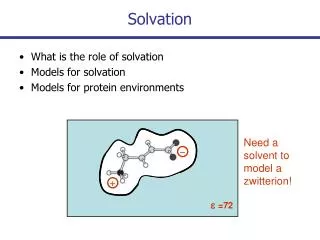
Solvation. What is the role of solvation Models for solvation Models for protein environments. Need a solvent to model a zwitterion!. -. +. e =72. Solvation. Solvation influences: Structure Energetics Spectroscopy Equilibria…. Free Energy of Solvation. To Solvate a Species:

Solvation
E N D
Presentation Transcript
Solvation • What is the role of solvation • Models for solvation • Models for protein environments Need a solvent to model a zwitterion! - + e =72
Solvation • Solvation influences: • Structure • Energetics • Spectroscopy • Equilibria…
Free Energy of Solvation • To Solvate a Species: • Making space for the solute molecule in the solvent; the enthalpy and entropy change needed to make a cavity in the solvent • Coupling the solute and the solvent energetically, ie including solute/solvent interaction terms through van der Waals and electrostatic interactions (and hydrogen bonding) • Relaxing the solvent and solute molecules
Free Energy of Solvation • DGsol the free energy change to transfer a molecule from vacuum to solvent. • DGsol = DGelec + DGvdw + DGcav (+ DGhb) An explicit hydrogen bonding term. Electrostatic component. Free energy required to form the solute cavity. Is due to the entropic penalty due to the reorganization of the solvent molecules around the solute and the work done in creating the cavity. Van der Waals interaction between solute and solvent.
Models for Solvation • Not at all • Implicit or continuum models • Explicit quantum models of hydration • Classical dynamical models of hydration • A combination of models
Continuum Methods • Solvent interactions are dominated by electrostatics • Treat electrostatics classically • Turn a quantum electron density into a classical charge distribution and solve the Poisson equation for interaction with a dielectric continuum
Continuum Models • In a dielectric medium the charge distribution of the solute polarises the dielectric and this induces a Reaction Field in the solute cavity • the Reaction Field interacts with the dipolar molecule by: • perturbing the rotational motion of the molecule causing it to have a preferred orientation • enlarging the dipole moment of the molecule by elastic displacement of its constituent charges. This induced dipole moment is denoted af, wherea is the polarizability of the molecule and f is the electric field acting on the molecule due to all sources except the molecule itself e m a
Dielectric The dielectric constant of a solvent is defined as the ability of the solvent to respond to an applied electric field:
Dielectric dielectric constant can be considered as the solvent’s ability to interact with a charged (or dipolar) solute : Charge in a nonpolar solvent Charge in a polar solvent e =2-4 e(water)=78; e(methanol)=40
Dielectric dielectric constant can be considered as the solvent’s ability to interact with a charged (or dipolar) solute : Dipole in a nonpolar solvent Dipole in a polar solvent e =2-4 e(water)=78; e(methanol)=40
The Born Model for Ion Solvation e a q • Born, 1920: the electrostatic component of the free energy of solvation for placing a charge in a spherical solvent cavity. • The solvation energy is equal to the work done to transfer the ion from vacuum to the medium. This is the difference in work to charge the ion in the two environments. • Ionic radii from crystal structures is used. • Only relevant for species with a formal charge.
Gruesome Details • Mathematical Formulas that can be applied • A rather complex procedure is used to determine the Born radii in Still’s implementation. In short, The Born radius of an atom corresponds to the radius that would return the electrostatic energy of the system according to the Born equation if all of the other molecules in the system were uncharged. • In Cramer and Truhlar’s QM approach the radius of the atom is a function of the charge on the atom.
The Onsager Model • Onsager, 1936: considers a polarizable dipole with polarizability a at the center of a sphere. • The solute dipole induces a reaction field in the surrounding medium which in turn induces an electric field in the cavity (reaction field) which interacts with the dipole.
The Onsager Model Onsager’s model assumes: • A molecule occupies a sphere of radius a, its polarizability, a, is isotropic, and no saturation(ie frequency dependent) effects can take place. • The short range molecular interaction energy is negligible compared to kBT. • The Onsager reaction field R is proportional to m and in the same direction as m
Classical Onsager Equation • If the species is charged an appropriate Born term must be added. • Other Models: A point dipole at the center of a sphere (Bell), A quadrupole at the center of a sphere (Abraham), multipole expansion to represent the solute, ellipsoidal and molecular cavities.
Quantum Onsager – Self Consistent Reaction Field • The reaction field is a first-order perturbation of the Hamiltonian. Correction factor corresponding to the work done in creating the charge distribution of the solute within the cavity in the medium
The Cavity in the Onsager Model • Spherical and ellipsoidal cavities may be used • Advantage: analytical expressions for the first and second derivatives may be obtained • Disadvantage: this is rarely true! • How does one define the radius value? • For a spherical molecule the molecular volume, Vm can be found: • Estimate by the largest interatomic distance • Use an electron density contour • Often the radius obtained from these procedures is increased to account for the fact that a solvent particle can not approach right up to the molecule
Surfaces Isodensity surface +
The Polarizable Continuum Method (PCM) • Scaled van der Waals radii of the atoms are used to determine the cavity surface. • The solute charge distribution is projected onto this surface as either a discretised distribution or a continuous distribution • For example: the surface is divided into a number of small surface elements with area DS. • If Ei is the electric field gradient at pt i due to the solute then an initial charge, qi is assigned to each element via: • The potential due to the point charges, fs(r) is found, giving a new electric field gradient. The charges are modified until they converge. • The solute Hamiltonian is modified: • After each SCF new values of qi and fs(r) are computed.
The PCM Approach Problems: • Using a discretised charge is problematic • The wavefunction extends outside the cavity so the sum of the charges on the surface is not equal and opposite to the charge of the solute outlying charge error • The charge distribution may be scaled so that this is true • The result depends upon the nature of the cavity and the nature of the surface chosen Work done in creating the charge distribution within the cavity in the dielectric medium.
The Conductor-Like Screening Model (COSMO) • The dielectic is replaced with a conductor: • For the classical case the energy of the system is: • C is the Coulomb matrix, • Bim represents the interaction between two unit charges placed at the position of the solute charge Qi and the apparent charge qm, and Amn represents the interaction between two unit charges at qm and qn.
SMD (Marenich, Cramer and Truhlar) • PCM model based on the generalized Born approximation • solvent cavity defined by superpositions of atom-centred spheres. • The “D” stands for “density” to denote that the full solute electron density is used without defining partial atomic charges. • This model includes “surface tension” terms at the solute−solvent boundary that are used model short-range interactions between the solute and solvent molecules in the first solvation shell. • The radii and the atomic surface tensions have been parametrized with a training set of 2821 solvation data including nonaqueous solvents • It gives significantly better results (especially for non-aqueous solvents) than the original PCM formalism.
Explicit inclusion of Solvent Molecules • the simplest and most accurate solvation model is to use collections of the actual solvent molecules for the solvent interactions performing a “supermolecule” calculation • BUT: typically many solvent molecules (100–1000) are required to adequately solvate a solute molecule • the expense of describing these molecules with quantum chemical techniques generally far outweighs the effort required to describe the substrate itself ! • Use MM for the solvent, giving a QM/MM method (BUT how many polarizable MM methods do we have…) • Embed the solute–solvent complex can be embedded in a periodic cell • Lots of solvent molecules introduce a large number of degrees of freedom that need to be either minimized or averaged over during the course of the calculation
Definitions of the First Solvation Shell… • predetermined number of solvent molecules, • a distance cutoff in the solute-solvent distribution functions • an energy cutoff in the size of the solute-solvent interaction energy. • those solvent molecules that make contact with the exposed van der Waals surface area of the solute • those components of the free energy that correlate statistically with the solvent accessible surface area or the van der Waals surface area
First Solvation Shell • Cavitation and dispersion (and hydrogen bonding) are the most important first solvation shell effects • stabilizing • a hydrogen bond can orient the solvent around a polar solute leading to a favourable interaction • destabilizing • the loss of orientational freedom (due to hydrogen bonding in the first solvation shell) around a nonpolar solute results in an unfavourable, hydrophobic interaction
2 water molecules • With 2 explicit water molecules, one to stabilize the positive and one to stabilize the negative charge, the minimum energy structures of the amino acids is zwitterionic. - +
Molecular Mechanics • Model the entire system classically using force fields “Mathematical expression describing the dependence of the energy of a molecule on all atomic coordinates” • there is no universally applicable water force field • the TIP4P water model is probably the most widely used
Composite Methods • Partition the system into QM/MM/Dielectric
Composite Methods • How are the partitions defined? • How is the coupling term between the partitions defined? • How is energy transferred between the partitions? • How sensitive are the results to the partitioning? • Gordon’s EFP method seems to be the most “self-consistent”
Effects of Solvent Solvent will preferentially stabilise: • solutes with bigger dipole moments • More polarisable solvents • Transition states tend to be more stabilised by solvent than reactants or produts • Solvent lowers energy barrier and speeds up the reaction • “Quantitative” accuracy requires accounting for first solvation shell effects • Typical accuracies are 10-20 kJ/mol
Solvent Effects on Spectra solution phase • Solvent has 2 main effects on absorption spectra: • absorption peaks become broader: gas phase • position oflmaxmay differ in different solvents: shift to longer l: ‘red shift’ shift to shorter l: ‘blue shift’
Protein Environments The hydrophobic side chains of a protein, illustrated as balls
Protein Environments the dipoles on the protein backbone
Protein Environments rotatable hydropholic side chains of a protein on the surface of a protein
Protein Environments a common partitioning of the dielectric