4.2 Context-Free Grammars
380 likes | 890 Vues
4.2 Context-Free Grammars. In this section, we shall introduce context-free grammars to generate a class of languages larger than the class of regular languages over the same alphabet. Definition 3: A context-free grammar (CFG) is denoted by G = (V, T, P, S), where.

4.2 Context-Free Grammars
E N D
Presentation Transcript
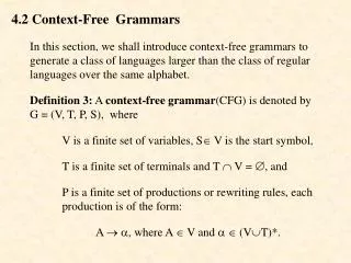
4.2 Context-Free Grammars In this section, we shall introduce context-free grammars to generate a class of languages larger than the class of regular languages over the same alphabet. Definition 3: A context-freegrammar(CFG) is denoted by G = (V, T, P, S), where V is a finite set of variables, S V is the start symbol, T is a finite set of terminals and T V = , and P is a finite set of productions or rewriting rules, each production is of the form: A , where A V and (VT)*.
Example 4: Let a CFG be G = (V, T, P, S), where V = {S}, T = {0, 1} and P contains the following productions: S 01 | 0S1 We have that S 01, S 0S1 0011, and S 0S1 00S11 000111. Therefore, S * 0 n1 n, for n = 1, 2, ....
Definition 4: The set generated by a context-free grammar G = (V, T, P, S) is { T* | S * } denoted by L(G). And L(G) is said to be a context-free language(CFL). If S * T*, then is said to be a sentence generated by the grammar G. We know that the set L = {0 n1 n | n = 1, 2, ....} is not regular. By definition 4 and example 4, L is context-free but not regular. Regular grammars are a special type of context-free grammars. Therefore, we have that the class of regular sets is a proper subset of the class of context-free sets over the same alphabet. Two grammars are equivalent if they generate the same set.
Example 5: The set of well-formed regular expressions over an alphabet, say = {0, 1}, is context-free. Solution : It is sufficient to show the rewriting rules as follows. S | | 0 | 1 | (S*) | (S+S) | (SS) Note: The definition of the set of productions is same as the recursive definition of regular expressions.
Example 6: Construct a CFG G such that L(G)= { {0, 1}* | = R}. Solution : S 0S0 | 1S1 | 0 | 1 | Example 7: Construct a CFG G such that L(G)= { R| {0, 1}* }. Solution : S 0S0 | 1S1 | We know that the set { R| {0, 1}* } is a subset of the set { {0, 1}* | = R}. And the difference is the set {0, 1}.
Given a CFL L, to construct a CFG G to generate L is not an easy job. Basically, there is no fixed method to solve the problem. If the language L is regular, it is quite easy. Usually, we can construct a regular grammar directly. Or by a DFA accepting the language, then convert to a regular grammar. For non-regular language, to construct a CFG G is more difficult. Most of time, we need to take care of the complicated recursive structure of the grammar. And we have to come to a case that a new defined variable must use previous defined variable in order to finish the recurrence. Sometimes, it could be easier if we construct a pushdown automaton M first, then convert the machine M to a CFG G. We have to wait until we reach chapter 5 to apply this method.
For some cases, we need to grasp the whole picture in order to construct a CFG. And sometimes, we may miss something. Example 8 : Construct a CFG G such that L = L(G) = { {0, 1}* | number of 0’s equal to number of 1’s in }. Solution :Method 1 : We may get a CFG G as follows. S 01S | 0S1 | S01 | 10S | 1S0 | S10 | But, how do we know the set generated by the grammar is what we want? We need to prove it by induction in most cases. Although, the grammar can generate strings with equal number of 1’s and 0’s, but can not generate the string 00111100. So, the grammar is not sufficient. What is the set generated by the above grammar?
Now, we need to modify the above grammar. Method 2 : Consider the following grammar : S 0S1S | 1S0S | The reason is that a string may start with 0, and 1 is somewhere after the symbol. And between 0 and 1 there are zero, one or more pairs of 0’s and 1’s. Similarly, after the pair of 0 and 1, there could be also many pairs of 0 and 1. If a string starts with 1, then the reason is similar. But, we only know that L(G) L. Before we prove that L L(G), we need to prove the following lemma first.
Lemma : If has nof 0‘s and n+1 of 1’s. Show that there exist a 1 such that = 1, and each of and has equal number of 0’s and 1’s, i.e., , L. Proof : Let = a 1 a 2 … a 2n+1, where a i is either 0 or 1. Define f(1) = 1, if a 1 = 0. Otherwise, f(1) = 1, as a 1 = 1. Define f(i+1) = f(i) 1, if a i = 0. Otherwise, f(i+1) = f(i) + 1, as a i = 1, for i = 1, 2, …, 2n. For 1 k 2n+1, let = a 1 a 2 … a k , then f(k) = number of 1’s in number of 0’s in . And f(k+1) is one greater than or less than f(k). If a 1 = 1, then = 1. We are done.
3 2 1 0 1 1 1 1 0 0 0 0 1 1 0 1 2 3 1 2 3 4 5 6 7 8 9 10 11 If a 1 = 0, then f(1) = 1. Since f(2n+1) = 1, there exist a smallest k, 3 k 2n+1, such that a k = 1, f(k) = 1 and f( j ) 1, for 1 j k . The value f(k1) must be 0, one less than f(k). Let = a 1 a 2 … a k-1. Then has equal number of 0’s and 1’s.Done! For instance, = 00101101110. Consider the graph of f(n). The value of f(1) is 1. We have f(8) = 0 and f(9) = 1, where a 9 = 1. And = 00101101 has equal number of 0’s and 1’s.
Now, we can show that L L(G) by induction as follows. (1) L, S * . Hence, L(G). (2) L, and | | = 2n, Assume that S * , L(G). (3) ’ L, and | ’ | = 2n+2. (a) Consider ’ = 0 L. Then has nof 0‘s and n+1 of 1’s. By lemma, there exists a 1 such that = 1, and each of and has equal number of 0’s and 1’s, i.e., , L. We have S 0S1S * 01S * 01 = ’ L(G). (b) Consider ’ = 1 L. Then has nof 1‘s and n+1 of 0’s. By the same reason as in (a), we have that S 1S0S * 10S * 10 = ’ L(G). Done!
Sometimes, we need to set up the recurrence as follows. Method 3 : Another solution for example 8. A required CFG is as follows. S 0B | 1A | B 1S | 0BB |1 A 0S | 1AA |0 The reason is that for any string , there are only 3 cases: (a) number of 0’s equal to number of 1’s in , let it be S. (b) number of 0’s is one more than number of 1’s in , let it be A. (c) number of 0’s is one less than number of 1’s in , let it be B.
Let consider the following steps: (1) L(G), we need a production S (2) If S * 0, we need S 0B, where B * , and has one more 1’s than 0’s. Mark B as a state with one extra 1’s. (3) If S * 1, we need S 1A, where A * , and has one more 0’s than 1’s. Mark A as a state with one extra 0’s. (4) If B * 1, then has equal number of 0’s and 1’s. Hence, we need B 1S | 1. The recurrence relation is set up. (5) If B * 0, then has 2 more 1’s than 0’s. Hence, we need B 0BB. The recurrence relation is set up. (6) The case for variable A is similar to the variable B. And we have that A 0 | 0S | 1AA. Done!
Example 9: Construct a CFG G such that L(G) =L= { {0, 1}* | number of 0’s is twice as many as number of 1’s in }. Solution : Method 1 : Consider the following CFG. S 0S0S1S | 0S1S0S | 1S0S0S | Question: Is L(G) = L?
Method 2 : Consider the following CFG. For any string , let n and m be the numbers of 0’s and 1’s in , respectively. Then there are only 5 cases: (a) n = 2m, let it be the state S. (b) n = 2m + 2, or (n 2) = 2m, let it be A. (c) n = 2m 1, or (n 1) = 2(m 1), let it be B. (d) n = 2m 2, or n = 2(m 1), let it be C. (e) n = 2m + 1, or, (n 1) = 2m, let it be D.
Let consider the following steps: (1) L(G), we do not need a production S (2) If S * 0, we need S 0B, where B * , and has one less 0 than twice as many 0’s as 1’s. Mark B as a state of one extra 0’s and one extra 1’s, or <1, 1> for short. (3) If S * 1, we need S 1A, where A * , and has two more 0’s than twice as many 0’s as 1’s. Mark A as a state of two extra 0’s, or <2, 0> for short. (4) If B * 0, we need B 0C, where C * , and has one more 1 than twice as many 0’s as 1’s. Mark C as a state of one extra 1’s, or <0, 1> for short. (5) If B * 1, we need B 1D, where D * , and has one more 0’s than twice as many 0’s as 1’s. Mark D as a state of one extra 0’s, or <1, 0> for short.
(6) If A * 0, we need A 0D. (7) If A * 1, we need A 1AA | 1DDDD | 1ADD | 1DAD | 1DDA. (8) If C * 1, we need C 1S | 1. (9) If C * 0, we need C 0BC | 0CB | 0CCD | 0CDC | 0DCC. (10) If D * 0, we need D 0S | 0. (11) If D * 1, we need D 1AD | 1DA | 1DDD.
The result is as follows. (1) S 0B | 1A. (2) B 0C | 1D. (3) A 0D | 1AA | 1DDDD | 1ADD | 1DAD | 1DDA. (4) C 1S | 1 | 0BC | 0CB | 0CCD | 0CDC | 0 DCC. (5) D 0S | 0 | 1AD | 1DA | 1DDD. We need to prove that L = L(G). Done!
Derivations and derivation trees(parse trees) Example 10: Consider the following grammar E E + E | E E | (E) | <integer> where the production of the variable <integer> is defined in section 4.1. Now, consider the derivation for E * 9 4 + 3. We use leftmost derivation, i.e., rewrite the leftmost variable, to get the derivations. E E E <integer> E * 9 E 9 E + E 9 <integer> + E * 9 4 + E 9 4 + <integer> * 9 4 + 3.
E E E Now, select a different production at the first step, we have E E + E E E + E <integer> E + E * 9 E + E 9 <integer> + E * 9 4 + E 9 4 + <integer> * 9 4 + 3. For a production E E E, a derivation E E E corresponds to a subtree of derivation (or parse) tree as follows. The variable E on the left side of the production is the root of the subtree, and the items on the right side of the production become the children of the root and listed in the same order as in the right side of the production.
E E E E + E <integer> * <integer> <integer> 9 * * 3 4 For derivations E * 9 4 + 3 as follows, we have a corresponding parse tree listed below. E E E <integer> E * 9 E 9 E + E 9 <integer> + E * 9 4 + E 9 4 + <integer> * 9 4 + 3.
E E E + E E <integer> * <integer> <integer> 3 * * 4 9 For derivations E * 9 4 + 3 as follows, we have a corresponding parse tree listed below. E E + E E E + E <integer> E + E * 9 E + E 9 <integer> + E * 9 4 + E 9 4 + <integer> * 9 4 + 3.
9 + 4 3 9 + 4 3 The above two parse trees correspond to the following two expression trees. The evaluation of the left tree is equal to 2, which is 9(4+3). The evaluation of the right tree is equal to 8, which is (94)+3. Therefore, the two parse trees of the derivations E * 9 4 + 3 are totally different. Actually, these two parse trees are not graphically isomorphic. And they possess different interpretation.
Definition 5: Let G = (V, T, P, S) be a context-free grammar. If there is a string T* and there are two different parse trees for the derivation S *, then the CFG G is said to be ambiguous. Example 11: Modify the following grammar E E + E | E E | (E) | <integer> to a new grammar E (E + E) | (E E) | <integer> Although we can eliminate the ambiguity of the first grammar, but sacrifice the convenience for dropping parentheses.
Left recursion and right recursion Example 12 : Let L ={20 n1 | n 0}. L is context-free. Consider the following grammar G 1. S A1 A A0 | 2 The production A A0 is a left recursive production, for instance S A1 A01 A001 A0001 A00001 20001
Consider the following grammar G 2. S A1 A 2 | 2B B 0 | 0B The production B 0B is a right recursive production, for instance S A1 2B1 20B1 200B1 20001 Left recursive productions can be modified to right recursive productions, and vise versa. The method to modify is shown by the following theorem. Definition 6: An A-production is a production with variable A on the left side.
Theorem 4 : Let G = (V, T, P, S) be a CFG. Let A A 1 | A 2 | … | A s be the set of left recursive A-productions. Let A 1 | 2 | … | t be the set of remaining A-productions. Let G’ = (V {B}, T, P’, S) be a CFG, where P’ = P \ {old A-productions of P} {new A-productions and B productions defined as follows} A 1 | 2 | … | t | 1 B | 2B | … | t B B 1 | 2 | … | s | 1 B | 2 B | … | s B Then L(G) = L(G’). Proof : Leave as an exercise.