Download
1 / 28
280 likes | 306 Vues
An Overview of Formal Mathematical Reasoning with applications to Digital System Verification. Ganesh C. Gopalakrishnan Computer Science, Univ of Utah, Salt Lake City, UT 84112 www.cs.utah.edu/formal_verification Supported by NSF Grant CCR-9800928 and a generous grant from Intel Corporation.

E N D
An Overview of Formal Mathematical Reasoningwith applications to Digital System Verification Ganesh C. Gopalakrishnan Computer Science, Univ of Utah, Salt Lake City, UT 84112 www.cs.utah.edu/formal_verification Supported by NSF Grant CCR-9800928 and a generous grant from Intel Corporation
Overview • Digital systems • Mostly computers • Often Finite State Machines or other special purpose memories or I/O peripherals • Play various roles • Need to specify what’s desired of them • Need to implement them economically • Get them to work!
Overview • How to unambiguously express what’s desired? • How to describe the implementation likewise? • What does “works correctly according to spec” mean? • How much does it cost to establish correctness? • Is it worth it? • Do users understand or notice the effect of correct operation? Do they react favorably? • Do manufacturers believe in doing it right at any cost? • Do lessons get reflected back into the design process?
Views of correctness • It often exhibits flashes of plausibility! • It boots NT • It runs w/o crashing for 2 weeks • It often does what the documentation says • It is a gold-standard of predictable behavior (but timing vagaries are annoying) • Its time-response is reasonably predictable • With “legal vectors,” it’s fine… but it is anybody’s guess what they are • … • It’s so reliable that we don’t even notice it!
Various precise lingo • Precision is in the eye of the beholder • Precision according to needs • Don’t just say it – be able to do something with what you say (machine readable) • Be able to trace all consequences of what you say (“what if” queries) • Precise can be too verbose (the list of all I/O vectors is a precise description but useless for human reasoning) • Be able to avoid saying the irrelevant • Be able to generalize and “round” what you say • What’s the sweet-spot of precision and reasoning convenience?
Logic versus Physics • A computer “does as much logic” as a falling apple “does Newtonian mechanics” • A computer is a mindless bit basher • A computer is an oscillator on steroids • A computer is a CMOS oven • … yet it curiously is the case that one can make sense of many things computers do using mathematical logic
Logic versus Physics • [Barwise] Logic is in some sense more fundamental than physics because logic is what rational inquiry is all about. There is an overwhelming intuition that the laws of logic are somehow more fundamental, less subject to repeal, than the laws of the land, or even the laws of physics. • We’ve of course come a long way since we declared that Socrates was mortal since he was a man and all men are mortal. According to Manna, Logic now plays a role similar to that played by Calculus in “Engineering”
About this course • I hope to take you through a segment of mathematical logic I know well • I hope to drive a few examples home so that you have something concrete to reflect on • I hope to set the stage for the (much more fun) course on tool usage to follow • I hope to learn a lot from teaching you!
Course Outline • Boolean Reasoning • Propositional logic • Being able to “pump out” only true sentences • Being able to “pump out” sentences to corroborate all truths • Is there an algorithm to do the above? • What’s its run-time like? • To truth through proofs • Well, that’s the “classical” way; other (more practical ways) include being able to produce truths via computations… • Boolean algebras • One of many “meanings” • Other meanings – decision diagrams
Propositional logic • Gives a formal notation to write down truths • The language consists of propositional variables that range over True and False • The language provides connectives (., +, and !) that allows one to compose propositions • Every sentence in the language has a meaning • Usually the meanings are in terms of Boolean algebras (value domains plus functions) • One can also build data structures (e.g. BDDs) representing these truths
Soundness and Completeness • One likes to have algorithmic means of proving all true assertions (completeness) • One likes to have only sound proof systems (never be able to prove false) • These attributes (soundness and completeness) are shared by many other formal mechanisms… not just logics. • For example, given a context-free grammar • S -> 0 S 1 | 1 S 0 | S S | Epsilon • And the claim that the grammar generates all sentences with equal #0 and #1, one can define • Soundness: no string with unequal 0s and 1s generated • Completeness: all strings of equal 0s and 1s are generated • Puzzle: how do we prove this for this CFG? • Hint: soundness is easy; completeness through induction.
Complexity Results • Various notions in propositional logic • Attributes of sentences • Valid: true under all variable-settings (interpretations) • Satisfiable: there is a variable-setting that makes the sentence true • The complexity of determining satisfiability is unknown (best known is O(2^n)). This is related to the famous “3-sat problem” which is “NP complete” • Basic property of the sat problem: • There is a non-deterministic algorithm to check satisfiability in polynomial-time (guess sat asg and check in poly time) • If a computer algorithm can perform Boolean satisfiability checking in polynomial-time, then several problems for which only exponential exact algorithms are known can be solved by simulating them on top of a sat solver, with only an added polynomial simulation cost.
Hilbert-style Axiomatizations • One axiomatization of propositional logic: • axiom scheme • p => (q => p) • s => (p => q) => (s=>p) => (s=>q) • ((!q=> !p) => (p=>q)) • rules of inference • only one: Modus ponens : a a => b ------------- b
Proofs via primitive inferences .vs.proofs via semantic reasoning Proof of p => p • p => (q => p) • s => (p => q) => (s=>p) => (s=>q) • ((!q=> !p) => (p=>q)) • Modus Ponens • p => ((p=>p) => p) • (p => ((p =>p) => p)) => ( ( p=> (p=>p)) => (p=>p) ) • MP gives (p => (p => p)) => (p => p) • (p => (p => p)) is an axiom • MP gives (p => p) • Modern thought: don’t do the primitive inferences if you can help it; instead, build a BDD and blow it away; if you get all paths going to the ‘1’ leaf, the fmla is a tautology.
Illustration of quantificationand modular design principles • Propositional logic is surprisingly versatile for modeling • Illustrated on a simple CMOS ckt design theory (Hoare) • Illustrates the notion of refinement preorders • Illustrates the construction of non-trivial equivalences • Illustrates the notion of invariants • Illustrates monotonicity • Illustrates the notion of safe substitutability Concrete modeling of the above illustrated using the PVS theorem-prover
w u z v x Existential Quantification is iterated disjunction, and models information hiding • “Advanced” Boolean reasoning • Expressing information hiding • R(u,v,x,z) = Exists w . (w=u.v) . (z=x+w) • To calculate the new relation R(u,v,x,z) , simply do the summation (0= u.v) . (z=x+0) + (1=u.v) . (z=x+1) i.e. z = uv + x (!u + !v) • Existential quantification is basically an iterated disjunction (over all the values of the domain)
Universal Quantification is the Dual of Existential; also is iterated conjunction; used to model correctness for all inputs • The dual of Existential: Universal • Exists x. P(x) = not(forall x. not(P(x))) • One use of “Forall”: Forall inputs. Spec(inputs) = Imp(inputs) • Example: The incorrect assertion Forall A, B. And(A,B) = Or(A,B) • This can be reduced to And(0,0) = Or(0,0) . And(0,1) = Or(0,1) . And(1,0) = Or(1,0) . And(1,1) = Or(1,1) T F F T = F
A simple theory of CMOS combinational ckt design (Hoare, ’88) How does one model a CMOS transistor? “Nothing models a transistor like a transistor (Lance Glasser)”. Nevertheless we will create Simplistic models just for the sake of illustration. g => s=d !g => s=d But, these are poor models… it doesn’t convey the notion of “drive” (good 0, good 1, etc.)
Hoare’s idea: Use three attributes Need for drive Consistency Drive dg + (s=d) g . dg . (!s + !d) => (ds = dd) g => s=d !g . dg . (s + d) => (ds = dd) dg + (s=d) !g => s=d (C, D, N)
1 Now, let’s build an inverter o, do i, di inv((i,di),(o,do)) = ntrans((i,di),(0,1),(o,do)) || ptrans((i,di),(1,1),(o,do)) where 0 ntrans((g,dg),(s,ds),(d,dd)) = dg + (s=d) ) g . dg . (!s + !d) => (ds = dd) , (g => s=d, ptrans((g,dg),(s,ds),(d,dd)) = , ) !g . dg . (s + d) => (ds = dd) dg + (s=d) (!g => s=d, and (C1,D1,N1) || (C2,D2,N2) = (C1/\C2, D1/\D2, N1/\N2) = ( i => o=0 /\ !i => o=1 , i.di => do /\ !i.di => do, (di+o).(di+ !o) ) = ( o = !i, di => do, di)
Now, let’s build a bad buffer buf((i,di),(o,do)) = ntrans((i,di),(1,1),(o,do)) || ptrans((i,di),(0,1),(o,do)) i.di. !o => do /\ !i.di. o => do, - i.e. when di asserted, do when (o != i) - so we can never prove do 1 o, do i, di 0
Circuit Equivalencefrom a practical perspective (C1,D1,N1) == (C2,D2,N2) exactly when 1,2,3 hold 1) C1=C2 2) C1.D1 = C2.D2 – drives match only in the legal - operating zone – C1 and C2 sort - of are like ‘invariants’ 3) C1.D1.N1 = C2.D2.N2 – need for drive only - in states where the - ckt is consistent and - produces drive (so some - of its drive need might - be satisfied by the ckt) A canonical representation for (C,D,N) under the above equivalence is (C, C.D, C.D => N)
Circuit “betterness” (C1,D1,N1) [= (C2,D2,N2) reads “ckt 2 is better than ckt1” means C1 = C2 -- same logic function C2.D2 => D1 – ckt2 provides more drive than ckt1 --whenever C2 is operating consistently C1.D1.N1 => N2 – ckt2 needs less drive than ck1 - whenever ckt1 is operating - consistently and is obeying its - role of providing drives
Circuit “betterness” • If ckt1 [= ckt2 and ckt2 [= ckt1, we have • ckt1 == ckt2 where == is as defined before. • [= is a preorder • reflexive • transitive • It is NOT anti-symmetric. Preorders are • nice because they allow us to establish • equivalences that are accommodative. • (The conjunction of a partial-order and its • inverse forces the identity equivalence relation • that is too constraining.)
Monotonicity = ability to substitute and preserve “goodness” If ckt1 [= ckt2 then we desire that ckt1 || ckt [= ckt2 || ckt This is indeed true of the Hoare ckt calculus. Monotonicity is an important design principle, truly capturing modularity and “substitutivity without surprises.” If we substitute a better component for an existing component, the whole system ends up to be no worse than the original.
Hiding If we want to hide a wire w from a ckt C, we generally do “exists w. C”. However, in terms of our (C,D,N) attributes, we do the following. Let Hw.C denote “hide w from C.” Hw. (C,D,N) = (Exists w . C, -- willing to settle for w=0 or -- w=1 in terms of consistency Exists w,dw . C.D, -- can only provide the weakest -- compromise drive over all w,dw Forall w,dw . C.D => N) -- the strongest need for -- drive (over all w,dw) must -- be met.
Discussion Problems • Prove that a transmission-gate is better than • (according to [= ) an N-type pass transistor. R’ (C1,D1,N1) = ( g => i=o, g.dg.(!s+!d) => di=do, dg+(i=o) ) (C2,D2,N2)=( g => i=o, g.dg => (di=do), dg+(i=o) ) R R is of the form P => Q, and R’ of the form P’ => Q where P’ => P. Thus R => R’. Q P’ P
Summary of Module 1 • It all began with Boole in the 1850s – people didn’t pay • attention even after Claude Shannon showed its merit • It took several tries before Boolean reasoning caught on • Need to tackle the complexity. • Surprisingly versatile: • we saw a design calculus that has • structural operators such as || and hiding, • the notion of improvement, • that improvements are preorders, and • that the improvement relation is • monotonic (preserved in contexts).