A Data-First Architecture for Unstructured Wireless Networks
530 likes | 702 Vues
A Data-First Architecture for Unstructured Wireless Networks. Michael Meisel. Ph.D. Dissertation ProspectusOctober 12, 2010. Unstructured Wireless Networks. Multi-hop No controlled mobility Topology can be highly dynamic Can be connected or disconnected

A Data-First Architecture for Unstructured Wireless Networks
E N D
Presentation Transcript
A Data-First Architecturefor Unstructured Wireless Networks • Michael Meisel Ph.D. Dissertation ProspectusOctober 12, 2010
Unstructured Wireless Networks • Multi-hop • No controlled mobility • Topology can be highly dynamic • Can be connected or disconnected • Examples: MANETs, VANETs, disruption-tolerant networks, combinations thereof
Goals • One architecture that will work on any unstructured network • Follow the Named Data Networking (NDN) philosophy • Data first: delivery based on “what”, not “where” • Get rid of holdovers from the wired domain
Current Paradigm • Provide data delivery from source to destination node • Treat connected and disconnected networks separately
Connected Nets: The Wired Approach • Each node is assigned an IP address • Applications communicate using destination IPs • The routing protocol finds a single best path from source to destination • At each hop along the path, the sender determines which single node (based on step 3) is allowed to forward the data
Issues with The Wired Approach • IP addresses lose their meaning, aggregatability in mobile nets • Applications care about data, not location • Finding, maintaining hop-by-hop paths is expensive • Pre-determined paths don’t take advantage of the broadcast nature of wireless
Alternative: Opportunistic Routing • Improvements: • Takes advantage of the broadcast nature of wireless • Shortcomings: • Focused on stationary mesh networks • Still dependent on IP addressing, location-based delivery • Examples: ExOR [1], MORE [2] [1] S. Biswas and R. Morris. ExOR: opportunistic multi-hop routing for wireless networks. ACM SIGCOMM Computer Communication Review, 35(4):144, 2005. [2] S. Chachulski, M. Jennings, S. Katti, and D. Katabi. Trading structure for randomness in wireless opportunistic routing. In SIGCOMM ’07, pages 169–180. ACM, 2007.
Disconnected Network Routing • Improvements: • Can take advantage of the broadcast nature of wireless • No IP addressing • Shortcomings: • Inefficient for connected networks (or network segments) • Examples: Epidemic routing [3], Spray and Wait [4] [3] A. Vahdat and D. Becker. Epidemic routing for partially-connected ad hoc networks. Technical Report CS-2000-06, Duke University, 2000. [4] T. Spyropoulos, K. Psounis, and C. S. Raghavendra. Spray and wait: an efficient routing scheme for intermittently connected mobile networks. In WDTN: SIGCOMM Workshop on Delay-Tolerant Networking, 2005.
NDN Architecture • Routing/forwarding is based on data names instead of node addresses
NDN Communication • (Optional Step 0: Use a routing protocol to announce names) • Step 1: An application sends an Interest packet containing a request for data by name. It can be flooded or routed. • Step 2: Any node that has the data can send a Data packet back towards the source of the Interest. Intermediate nodes cache the data. • Future Interests for the same name can be serviced by caches
ucla/home Responder Requester ucla/home Interest Assume we flood Interests. 22
Responder Requester By forwarding the Interests, the intermediate nodes have established a path from responder to requester. 22
ucla/home Responder Requester Data The nodes that forward the data also cache it. 22
ucla/home Requester ucla/home Interest Suppose another node requests the same data name. 22
ucla/home Requester Responder ucla/home Responder Data Its immediate neighbors have cached the appropriate data, so they can respond. 22
NDN Advantages for Unstructured Nets • Applications can communicate based on data names only, no need to worry about location • Unlike IP addresses, data names are always meaningful • Built-in caching for disconnected networks • Can interoperate with wired NDN infrastructure
What is LFBL? • A forwarding protocol for connected wireless networks • A proof-of-concept for NDN in multi-hop wireless networks
LFBL Goals • Name-based communication at the application layer • Broadcast-only communication at the MAC layer • No control packets • Use the best available path on the fly • No path selection in advance
Communication • At first, requests are flooded • Requests contain the desired name • Any number of responders may respond with a data packet • Responses take the best available path back to the requester • Further requests for the same name take the best available path to the responder(s)
Broadcast-Only Forwarding • Forwarding decisions must be made by the receiver • Step 1: Determine if I am eligible to forward the packet. If so: • Step 2: Listen to see if another node closer to the intended destination forwards the packet. If not: • Step 3: Forward the packet
Follow-up Questions • How does a receiver know if it’s eligible to forward? • How long should a receiver listen, waiting for someone else to forward?
Distances and Eligibility • The network shares a single distance metric • (Could be: hop count, receive power, geo distance...) • In every packet, senders broadcast their distance to the requester and/or responder • Nodes track their distance to active endpoints • Only nodes closer to the destination are eligible forwarders
Listening Periods • Eligible forwarders choose their listening period based on the network’s delay metric • Tells the node how long to wait before forwarding • Only forward if a closer node does not forward before the listening period is over
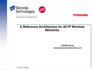
R broadcasts a request, all nodes forward, record their distance from R d(A,R) = 10 A d(E,R) = 3 d(B,R) = 8 E d(S,R) = 14 B S R d(F,R) = 3 F d(C,R) = 10 C d(D,R) = 16 D
S broadcasts a response. D will never forward. A, B, or C may forward... after some delay. d(A,R) = 10 A d(B,R) = 8 E d(S,R) = 14 B S R F d(C,R) = 10 C d(D,R) = 16 16 > 14 ineligible D
The delay depends on the network’s delay metric. d(A,R) = 10 A wait = ? d(B,R) = 8 E d(S,R) = 14 B S R wait = ? F d(C,R) = 10 C wait = ? D
Simplest delay metric: random. A wait = random() E B S R wait = random() F C wait = random() D
But the receivers have some useful information: their own distance to R and S’s distance to R. d(A,R) = 10 A d(B,R) = 8 E d(S,R) = 14 B S R F d(C,R) = 10 C D
C can calculate its listening period by comparing S’s claimed distance to R with its own prediction, assuming the packet were to travel through C. Its listening period will be proportional to the difference. A E d(S,R) = 14 B S R 5 F C distance traversed from S = 5 d(C,R) = 10 d(S,C,R) = 5+10 = 15 wait ∝ 15-14 D
Suppose all neighbors received the packet. B will forward immediately. A wait ∝ 1 (same as C) E B S R distance traversed from S = 6 d(C,R) = 8 d(S,R) = 6+8 = 14 wait ∝ 14-14 F C wait ∝ 1 D
A and C hear B before their listening period ends, so they do not forward. A E B S R F C D
Suppose B moved away. B A E B S R F C D
A and C will forward the packet instead, once their listening period is over. B A wait ∝ 1 E S R F C wait ∝ 1 D
But A and C will try to forward at the same time, resulting in a collision! B A wait ∝ 1 E S R F C wait ∝ 1 D
Simple solution: include a random factor as well. Suppose y < x. C will forward first, A will overhear and not forward. B A x = random() wait += x E S R F C y = random() wait += y D
Preliminary Handling of Stale State • Distances will become stale, discard old ones • Track variance in distance change • Make nodes with greater variance have longer listening periods • Allows us to implicitly prefer more stable paths
Simulation Setup • QualNet simulator • 100 nodes • 1500 x 1500 meter area • Random waypoint using steady-state initialization [5] • Bidirectional traffic; one request-response every 100 ms; multiple node pairs [5] W. Navidi and T. Camp. Stationary distributions for the random waypoint mobility model. Mobile Computing, IEEE Transactions on, 3(1):99 – 108, Jan 2004.
Evaluation Metrics • Roundtrip time: Time from request sent to response received • Response ratio: Responses received over requests sent • Overhead: Percent of bytes transmitted not in direct service of data delivery • Path length: Average length of all paths used for successful data delivery • Total data transferred:Total number of bytes successfully received at all endpoints (requesters and responders)
Problems with Stale State Request Interval (seconds)
Goal 1: Caching Support • Purpose: • Can improve performance in connected networks • Necessary to support disconnected networks • Challenges: • Will require significant changes to how LFBL deals with names • Selection of cache replacement algorithm