Download
1 / 30
310 likes | 460 Vues
Gene finding with GeneMark.HMM (Lukashin & Borodovsky, 1997 ). CS 466 Saurabh Sinha. Gene finding in bacteria. Large number of bacterial genomes sequenced (10 at the time of paper, 1997) Previous work: “Genemark” program identified gene as ORF that looks more like genes than non-genes.

E N D
Gene finding with GeneMark.HMM(Lukashin & Borodovsky, 1997) CS 466 Saurabh Sinha
Gene finding in bacteria • Large number of bacterial genomes sequenced (10 at the time of paper, 1997) • Previous work: “Genemark” program identified gene as ORF that looks more like genes than non-genes. • Uses Markov chains of coding and non-coding sequence • 5’ (starting) boundary not well predicted • Resolution of start point ~ 100 nucleotides
Genemark.hmm • Builds on Genemark, but uses HMM for better prediction of start and stop • Given DNA sequence S = {b1,b2,….bL} • Find “functional sequence” A={a1,…aL} where each ai = 0 if non-coding, 1 if coding in forward strand, 2 if coding in reverse strand • Sounds like the Fair Bet Casino problem (sequence of coin types “fair” or “biased”) • Find Pr(A | S) and report A that maximizes this
Functional sequence • “A” carries information about where the coding function switched into non-coding (stop of gene) and vice versa. • Model sequence by HMM with different states for “coding” and “non-coding” • Maximum likelihood “A” is the optimal path through the HMM, given the sequence • Viterbi algorithm to solve this problem
Hidden Markov Model • In some states, choose (i) a length of sequence to emit and (ii) the sequence to emit • This is different from the Fair Bet Casino problem. There, each state emitted exactly one observation (H or T)
Hidden Markov Model • “Typical” and “Atypical” gene states (one for each of forward and reverse strands) • These two states emit coding sequence (between and excluding start and stop codons) with different codon usage patterns • Clustering of E. coli genes showed that • majority of genes belong to one cluster (“Typical”) • many genes, believed to have been “horizontally transferred” into the genome, belong to another cluster (“Atypical”)
Hidden State Trajectory “A” • This is similar to the “functional” sequence defined earlier • except that we have one for each state, not one for each nucleotide • Sequence of M hidden states ai having duration di: • A = {(a1d1), (a2d2), …. (aMdM)} • ∑di = L • Find A* that maximizes Pr(A|S)
Formulation • Find trajectory (path) A that has the highest probability of occurring simultaneously with the sequence S • Maximizing Pr(A,S) is the same as maximizing Pr(A|S). Why ?
Solution • Maximization problem solved by Viterbi algorithm (seen in previous lecture)
Solution maximizing over all possible trajectories
Solution transition prob. Define (for dynamic progamming): prob. of duration prob. of sequence the joint probability of a partial trajectory of m states (with the last state being am) and a partial sequence of length l.
Parameters of the HMM • Transition probability distributions, emission probability distributions • Fixed a priori • What was the other possibility ? • Learn parameters from data • Emission probabilities of coding sequence state obtained from previous statistical studies: “What does a coding sequence look like in general?” • Emission probabilities of non-coding sequence obtained similarly
Parameters of the HMM • Probability that a state “a” has duration “d” (i.e., length of emission is d) is learned from frequency distribution of lengths of known coding sequences
Parameters of the HMM • … and non-coding sequences
Parameters of the HMM • Emission probabilities of start codon fixed from previous studies • Pr(ATG)=0.905, Pr(GTG)=0.090, Pr(TTG)=0.005 • Transition probabilities: Non-coding to Typical/Atypical coding state = 0.85/0.15
Post-processing • As per the HMM, two genes cannot overlap. In reality, genes may overlap ! G2 G1
Post-processing • As per the HMM, two genes cannot overlap. In reality, genes may overlap ! G2 G1 Will predict second gene to begin here What about the start codon for that second gene?
Post-processing • As per the HMM, two genes cannot overlap. In reality, genes may overlap ! G2 G1 • Look for an RBS somewhere here. • Take each start codon here, and find RBS -19 to -4 bp upstream of it
How to search for RBS? • Take 325 genes from E. coli (bacterium) with known RBS • Align them using sequence alignment • Use this as a PWM to scan for RBS
Gene prediction in different species • The coding and non-coding state emission probabilities need to be trained from each species for predicting genes in that species
Gene prediction accuracy • Data set #1: all annotated E. coli genes • Data set #2: non-overlapping genes • Data set #3: Genes with known RBS • Data set #4: Genes with known start positions
Results VA: Viterbi algorithm PP: With post-processing
Results • Gene overlap is an important factor • Performance goes up from 58% to 71% when overlapping genes are excluded from data set • Post-processing helps a lot • 58% --> 75% for data set #1 • Missing genes: “False negatives” < 5% • “Wrong” gene predictions: “False positives” ~8% • Are they really false positives, or are they unannotated genes?
Results • Compared with other programs
Results • Robustness to parameter settings • Alternative set of transition probability values used • Little change in performance (~20% change in parameter values leads to < 5% change in performance)
Higher Order Markov models • Sequence emissions were modeled by a second order Markov chain. • Pr (Xi|Xi-1, Xi-2,…X1) = Pr (Xi|Xi-1, Xi-2) • Examined the effect of changing the “Markov order” (0,1,3,4,5) • Even zeroth order Markov chain does pretty well.