Valuing Cash Flows
Valuing Cash Flows. Non-Contingent Payments. Non-Contingent Payouts. Given an asset with fixed payments (i.e. independent of the state of the world), the asset’s price should equal the present value of the cash flows. . Treasury Notes.

Valuing Cash Flows
E N D
Presentation Transcript
Valuing Cash Flows Non-Contingent Payments
Non-Contingent Payouts • Given an asset withfixed payments (i.e. independent of the state of the world), the asset’s price should equal the present value of the cash flows.
Treasury Notes • US Treasuries notes have maturities between 2 and ten years. • Treasury notes make biannual interest payments and then a repayment of the face value upon maturity • US Treasury notes can be purchased in increments of $1,000 of face value.
Consider a 3 year Treasury note with a 6% annual coupon and a $1,000 face value. $30 $30 $30 $30 $30 $1,030 Now 6mos 1yrs 1.5 yrs 2yrs 2.5yrs 3yrs F(0,1) F(1,1) F(2,1) F(3,1) F(4,1) F(5,1) F(0,1) = 2.25% You have a statistical model that generates the following set of (annualized) forward rates F(1,1) = 2.75% F(2,1) = 2.8% F(3,1) = 3% F(4,1) = 3.1% F(5,1) = 4.1%
$30 $30 $30 $30 $30 $1,030 Now 6mos 1yrs 1.5 yrs 2yrs 2.5yrs 3yrs 2.25% 2.75% 2.8% 3% 3.1% 4.1% Given an expected path for (annualized) forward rates, we can calculate the present value of future payments. + … $30 $30 $30 P = + + (1.01125) (1.01125)(1.01375) (1.01125)(1.01375)(1.014) + … $1,030 = $1,084.90 + (1.01125)………….(1.0205)
Forward Rate Pricing Cash Flow at time t Current Asset Price Interest rate between periods t-1 and t
Alternatively, we can use current spot rates from the yield curve $30 $30 $30 $30 $30 $1,030 Now 6mos 1yrs 1.5 yrs 2yrs 2.5yrs 3yrs
The yield curve produces the same bond price…..why? $30 $30 $30 $30 $30 $1,030 Now 6mos 1yrs 1.5 yrs 2yrs 2.5yrs 3yrs $30 $30 $30 $30 $30 $1,030 P = + + + + + 2 3 4 5 6 (1.0125) (1.0125) (1.0135) (1.0135) (1.015) (1.015) S(1) S(2) S(3) 2 2 2 P = $1,084.90
Spot Rate Pricing Current Asset Price Cash flow at period t Current spot rate for a maturity of t periods
Alternatively, given the current price, what is the implied (constant) interest rate. $30 $30 $30 $30 $30 $1,030 Now 6mos 1yrs 1.5 yrs 2yrs 2.5yrs 3yrs $30 $30 $30 $30 $30 $1,030 P + + + + + = 2 3 4 5 6 (1+i) (1+i) (1+i) (1+i) (1+i) (1+i) (1+i) = 1.015 (1.5%) P = $1,084.90 Given the current ,market price of $1,084.90, this Treasury Note has an annualized Yield to Maturity of 3%
Yield to Maturity Cash flow at time t Yield to Maturity Current Market Price
Yield to maturity measures the total performance of a bond from purchase to expiration. Consider $1,000, 2 year STRIP selling for $942 .5 $1,000 $1,000 1.03 (3%) $942 = (1+Y) = = $942 2 (1+Y) For a discount (one payment) bond, the YTM is equal to the expected spot rate For coupon bonds, YTM is cash flow specific
Consider a 5 year Treasury Note with a 5% annual coupon rate (paid annually) and a face value of $1,000 The one year interest rate is currently 5% and is expected to stay constant. Further, there is no liquidity premium Yield 5% Term $50 $50 $50 $50 $50 P + + + + = = $1,000 2 3 4 5 (1.05) (1.05) (1.05) (1.05) (1.05) This bond sells for Par Value and YTM = Coupon Rate
Consider a 5 year Treasury Note with a 5% annual coupon rate (paid annually) and a face value of $1,000 Now, suppose that the current 1 year rate rises to 6% and is expected to remain there Yield 6% 5% Term $50 $50 $50 $50 $50 P + + + + = = $958 2 3 4 5 (1.06) (1.06) (1.06) (1.06) (1.06) This bond sells at a discount and YTM > Coupon Rate
Price A 1% rise in yield is associated with a $42 (4.2%) drop in price $1,000 $42 $958 Yield 5% 6%
Consider a 5 year Treasury Note with a 5% annual coupon rate (paid annually) and a face value of $1,000 Now, suppose that the current 1 year rate falls to 4% and is expected to remain there Yield 5% 4% Term $50 $50 $50 $50 $50 P + + + + = = $1045 2 3 4 5 (1.04) (1.04) (1.04) (1.04) (1.04) This bond sells at a premium and YTM < Coupon Rate
Price A 1% drop in yield is associated with a $45 (4.5%) rise in price $1,045 $45 $1,000 $42 $958 Yield 4% 5% 6%
A bond’s pricing function shows all the combinations of yield/price Price • The bond pricing is non-linear • The pricing function is unique to a particular stream of cash flows $1,045 $45 $1,000 $42 $958 Pricing Function Yield 4% 5% 6%
Duration • Recall that in general the price of a fixed income asset is given by the following formula • Note that we are denoting price as a function of yield: P(Y).
For the 5 year, 5% Treasury, we had the following: Yield 5% Term $50 $50 $50 $50 $50 P(Y=5%) = + + + + = $1,000 2 3 4 5 (1.05) (1.05) (1.05) (1.05) (1.05) This bond sells for Par Value and YTM = Coupon Rate
Price $1,000 Pricing Function Yield 5%
Suppose we take the derivative of the pricing function with respect to yield For the 5 year, 5% Treasury, we have
Now, evaluate that derivative at a particular point (say, Y = 5%, P = $1,000) For every 100 basis point change in the interest rate, the value of this bond changes by $43.29 This is the dollar duration DV01 is the change in a bond’s price per basis point shift in yield. This bond’s DV01 is $.43
Price Duration predicted a $43 price change for every 1% change in yield. This is different from the actual price Error = $2 $1,045 $1,000 Error = - $1 $958 Pricing Function Yield 4% 5% 6% Dollar Duration
Dollar duration depends on the face value of the bond (a $1000 bond has a DD of $43 while a $10,000 bond has a DD of $430) modified duration represents the percentage change in a bonds price due to a 1% change in yield For the 5 year, 5% Treasury, we have Every 100 basis point shift in yield alters this bond’s price by 4.3%
Macaulay's Duration Macaulay’ duration measures the percentage change in a bond’s price for every 1% change in (1+Y) (1.05)(1.01) = 1.0605 For the 5 year, 5% Treasury, we have
For bonds with one payment, Macaulay duration is equal to the term Dollar Duration Example: 5 year STRIP Modified Duration Macaulay Duration
Think of a coupon bond as a portfolio of STRIPS. Each payment has a Macaulay duration equal to its date. The bond’s Macaulay duration is a weighted average of the individual durations Back to the 5 year Treasury $50 $50 $50 $50 $50 P(Y=5%) = + + + + = $1,000 (1.05) 2 3 4 5 (1.05) (1.05) (1.05) (1.05) $47.62 $45.35 $43.19 $41.14 $822.70 $47.62 $45.35 $43.19 $41.14 $822.70 1 + 2 + 3 + 4 + 5 $1,000 $1,000 $1,000 $1,000 $1,000 Macaulay Duration = 4.55
Macaulay Duration = 4.55 Macaulay Duration Modified Duration = (1+Y) 4.55 Modified Duration = = 4.3 1.05 Dollar Duration = Modified Duration (Price) Dollar Duration = 4.3($1,000) = $4,300
Duration measures interest rate risk (the risk involved with a parallel shift in the yield curve) This almost never happens.
Yield curve risk involves changes in an asset’s price due to a change in the shape of the yield curve
Key Duration • In order to get a better idea of a Bond’s (or portfolio’s) exposure to yield curve risk, a key rate duration is calculated. This measures the sensitivity of a bond/portfolio to a particular spot rate along the yield curve holding all other spot rates constant.
Returning to the 5 Year Treasury A Key duration for the three year spot rate is the partial derivative with respect to S(3) Evaluated at S(3) = 5%
Key Durations X 100 Note that the individual key durations sum to $4329 – the bond’s overall duration
Yield Curve Shifts +1% 0% - 2% - 4% +1%
+1% 0% - 2% - 4% +1% $.4535 1 + $.8638 1 + $.12341 0 + $.15671 (-2) + $39.81 (-4) = $161 This yield curve shift would raise a five year Treasury price by $161
Suppose that we simply calculate the slope between the two points on the pricing function Price $1,045 - $958 Slope = = $43.50 4% - 6% $1,045 or $1,045 - $958 *100 $1,000 = 4.35 Slope = $958 4% - 6% Yield 4% 6%
Effective duration measures interest rate sensitivity using the actual pricing function rather that the derivative. This is particularly important for pricing bonds with embedded options!! Price $1,045 Effective Duration $958 Pricing Function Yield 4% 6% Dollar Duration
Value At Risk Suppose you are a portfolio manager. The current value of your portfolio is a known quantity. Tomorrow’s portfolio value us an unknown, but has a probability distribution with a known mean and variance Profit/Loss = Tomorrow’s Portfolio Value – Today’s portfolio value Known Distribution Known Constant
Probability Distributions 1 Std Dev = 65% 2 Std Dev = 95% 3 Std Dev = 99% One Standard Deviation Around the mean encompasses 65% of the distribution
Remember, the 5 year Treasury has a MD 0f 4.3 $1,000, 5 Year Treasury (6% coupon) Interest Rate Mean = $1,000 Std. Dev. = $86 Mean = 6% Std. Dev. = 2% Profit/Loss Mean = $0 Std. Dev. = $86
The VAR(65) for a $1,000, 5 Year Treasury (assuming the distribution of interest rates) would be $86. The VAR(95) would be $172 In other words, there is only a 5% chance of losing more that $172 1 Std Dev = 65% 2 Std Dev = 95% 3 Std Dev = 99% One Standard Deviation Around the mean encompasses 65% of the distribution
A 30 year Treasury has a MD of 14 $1000, 30 Year Treasury (6% coupon) Interest Rate Mean = $1,000 Std. Dev. = $280 Mean = 6% Std. Dev. = 2% Profit/Loss Mean = $0 Std. Dev. = $280
The VAR(65) for a $1,000, 30 Year Treasury (assuming the distribution of interest rates) would be $280. The VAR(95) would be $560 In other words, there is only a 5% chance of losing more that $560 One Standard Deviation Around the mean encompasses 65% of the distribution
Example: Orange County • In December 1994, Orange County, CA stunned the markets by declaring bankruptcy after suffering a $1.6B loss. • The loss was a result of the investment activities of Bob Citron – the county Treasurer – who was entrusted with the management of a $7.5B portfolio
Example: Orange County • Actually, up until 1994, Bob’s portfolio was doing very well.
Example: Orange County • Given a steep yield curve, the portfolio was betting on interest rates falling. A large share was invested in 5 year FNMA notes.
Example: Orange County • Ordinarily, the duration on a portfolio of 5 year notes would be around 4-5. However, this portfolio was heavily leveraged ($7.5B as collateral for a $20.5B loan). This dramatically raises the VAR
Example: Orange County • In February 1994, the Fed began a series of six consecutive interest rate increases. The beginning of the end!
Risk vs. Return • As a portfolio manager, your job is to maximize your risk adjusted return Risk Adjusted Return = Nominal Return – “Risk Penalty” You can accomplish this by 1 of two methods: 1) Maximize the nominal return for a given level of risk 2) Minimize Risk for a given nominal return

