Stochastic Models for Gene Expression: Understanding Fluctuations in Biological Networks
This presentation discusses the significance of stochastic models in gene expression and their application to biology, particularly focusing on the fluctuations present in gene networks. The talk covers fundamental concepts, including the dynamics of molecular networks, the role of epigenetic variability, and the impact of noise on gene expression. It explores advanced models, such as the Gillespie algorithm and hybrid approaches, emphasizing the interplay between discrete and continuous dynamics. The implications for understanding molecular interactions and the challenges of analytical solutions will also be highlighted.

Stochastic Models for Gene Expression: Understanding Fluctuations in Biological Networks
E N D
Presentation Transcript
Stochastic models for gene expressionOvidiu Radulescu, DIMNP UMR 5235, Univ. of Montpellier 2Colloque franco-roumain mathématiques appliquées, Poitiers 29/08/10
Summary • Motivation : fluctuations in gene networks • Stochastic models for gene expression • Application to biology: fluctuome
From genes to gene networks Interactions between genes, proteins, metabolites From genes to proteins Gene networks, feed-back
Fluctuations in molecular networks Epigenetic variability Intermittent protein production Becksai et al EMBO J 2001: S.cerevisiae Cai et al. Nature 2006: beta-gal operon Ozbudak et al Nature 2002: one promoter noise in B.subtilis Which is the origin of fluctuations? Is there some order/logics in randomness? Questions to answer
How to tame fluctuations? either all numbers large, or all small numbers fast G P k2 k1 Fast The central limit theorem and the law of large numbers: if the number of molecules is large for ALL molecular species, then the fluctuations are small and Gaussian; dynamics is close to deterministic The averaging theorem: if a slow deterministic system receives rapid random fluctuations as input then the output has small fluctuations
Noise in multiscale networks with inverted time hierarchy Low and large numbers : a broad distribution of abundances from a few to 104 per cell Multiscale Fast and slow processes : from 10-3 to 104 s Inverted time hierarchy: some processes involving low numbers are slow G P k2 k1 Slow Hybrid noise : discrete variations of low numbers species, continuous variation punctuated by jumps or switching of large numbers species
Delbrück-Rényi-Bartolomay approach Which reaction? Which time? Generate exponential variable of parameter (k1A+k2B) • Dynamics variables are numbers of molecules of different species • All species evolve by discrete jumps separated by random waiting times Two main assumptions: • Reactions are independent; • Transport is instantaneous. Gillespie’s algorithm Disadvantages: • Time costly • Analytical solutions of the Chemical Master Equation are rarely available
Continuous time Markov jump processes are n chemical species is the state biochemical reaction jump vector intensity distribution of jumps jump probability
Hybrid approach Which time? Generate exponential variable of parameter (k1A+k2B)-1 • 2 types of dynamical variables: discrete and continuous • Discrete variables undergo random jumps, continuous variables follow ODE dynamics Assumption: • Law of large numbers can be applied to continuous variables • Gaussian noise neglected Discrete variable : Gillespie dynamics Hybrid algorithm Advantages: • Slight improvement of execution time • Emphasize the hybrid nature of fluctuations • Analytical solutions more easily available Continuous variable : ODE switching The hybrid stochastic dynamics is a piecewise deterministic Markov process
Partial fluid approximation:partition Given a pure jump model, find its hybrid approximation Species partition: discrete, continuous Reaction partition Discrete transitions coupling intrinsic Contributions to continuous flow Coupling between discrete and continuous only if super-reactions of type 1: fast, change mode XC, rates depend on XD switching
Partial fluid approximation : expansion Rescaling 1st order Taylor expansion in Chemical Master Equation Switching Hybrid Master/Fokker-Planck equation of a PDP with switching Drift Coupling if super-reactions of type 1
Partial fluid approximation : breakage breakage super-reactions of type 2: very fast, act on XC, rates depend on XD e fast back to ground discrete reactions breakage frequency breakage size distribution Breakage+drift part in the master/Fokker-Planck equation
Hierarchical model reduction Which time? Generate exponential variable of parameter (k1A+k2B)-1 • Eliminate inessential details: pruning • Group together reactions: lumping • Zoom in and out complexity • Drastic decrease of simulation time Reduction of stochastic models: • Linear sub-networks • Needs multi-scaleness • Works both for deterministic and for stochastic models k2 A2 k1 Aj A1 k kklim/ki Ai Aj klim ki A k<<ki At Dominance and pruning Un-broken cycle: averaging
Inverted time hierarchies • Stochastic leaks of low mass un-broken cycles produces slow transitions of discrete variables, thus inverted time hierarchies k2 A2 k1 Aj A1 k kklim/ki Ai Aj klim ki A k<<ki At A un-broken cycle can be a source of hybrid noise • Low intensity shot noise is amplified to bursts by fast transitions of the continuous variables kklim/ki kp Burst amplification kp>>kd Aj A B Discrete variables kd Continuous variable
D** model1 model2 model3 1.5e-4 k1=400 D** TrRNAP Inverted time hierarchy D D.R 1.5e-4 0.3 km1=1 TrRNAP k2=6 km2=10 Burst amplification of ElRib 1e-2 RBS* Ø Ø 0.3 D.RNAP 0.5 0.3 RBS Ø k3=0.1 1e-5 0.015 1.3e-4 ElRib Prot FoldedProt TrRNAP 2.25 60 Continuous variables k4=0.3 Rib.RBS Ø Ø RBS 0.5 k5=0.3 1e-5 0.015 1.3e-4 km6=2.25 k6=60 ElRib Prot FoldedProt Ø Ø Rib.RBS k7=0.5 k10=1e-5 k11=1e-5 k9=1.3e-4 Hierarchical model reduction k8=0.015 ElRib Prot FoldedProt
Hierarchical model reduction: gain in computational power Crudu et al BMC Systems Biology 2009
A simple model : solution of the hybrid master/Fokker-Planck equation Gamma steady state distribution • a=k1/g2 : number of transcription initiations per protein lifetime • b=k2/g1 : number of proteins per burst
Biological system: central carbon metabolism in B.subtilis Bacteria are grown in two experimental conditions: glucose-rich and malate-rich medium
Experimental method: number and brightness Poissonian field F map Histograms
Part of the fluctuome: CggR, gapB, CcpN Malate Malate 10min Glucose 60min CcpN Glucose Glucose CggR gapB Malate Matthew Ferguson, CBS
RNAP RNAP B A gapB k3 or k3’ k1on RNAP RNAP RNAP RNAP D D.R D.RNAP CggR TrRNAP RBS bursting RNAP CggR CcpN CggR k1off RNAP RNAP k6 D k3 k3’ RNAP k1on k6 RNAP k4’ pcggR RNAP RNAP TrRNAP RNAP RNAP k4 pRNAP-R Ø RNAP RNAP D.R.RNAP RBS D.RNAP TrRNAP paused k4’~0 TrRNAP k1off RBS bursting k4 k5 RNAP RBS RNAP RNAP Ø C k7 ElRib k8 pgapB MdGFP Ø kdeg
Take home message • The origin of noise in multiscale molecular network is the inverted time hierarchy; noise is hybrid • Hierarchical model reduction unravels functional structure: unbroken cycles, burst amplifiers, integrators • Noise carries information about interactions : fluctuome could be an important tool
Acknowledgements Nathalie Declerck, Matthew Ferguson, Catherine Royer CBS Montpellier Alina Crudu, Arnaud Debussche, Aurelie Muller IRMAR Rennes, ENS Cachan Alexander Gorban University of Leicester