Download
1 / 17
170 likes | 322 Vues
A few longitudinal BBU simulations (in the SPL case) J-Luc Biarrotte CNRS, IPN Orsay. HOM excitation analyses. Beam flying ONCE through 1 cavity Allows to study when a HOM mode hits a beam spectrum resonance line Analytical power analysis is possible (& sufficient)

E N D
A few longitudinal BBU simulations (in the SPL case)J-Luc BiarrotteCNRS, IPN Orsay
HOM excitation analyses • Beam flying ONCE through 1 cavity • Allows to study when a HOM mode hits a beam spectrum resonance line • Analytical power analysis is possible (& sufficient) • Beam flying ONCE through N cavities • Allows also to study if a Beam Break-Up (BBU) rises « out from the noise » • Simulation is required (with very consuming CPU time) • (Beam flying N times through 1 cavity) • Non-Applicable to linacs
Input parameters for the SPL case • PROTON BEAM • 352.2 MHz, 50 Hz, 5% d.c. (1ms pulse) • 150 MeV input energy • 400 mA mean pulse current • SC LINAC • 150 cavities @704.4 MHz • 20.7MV acc.voltage, -15° synch.phase (-> 3.15 GeV) • HOM mode considered: • 2000 MHz (far from main beam resonances) • Q=1E8 (no HOM coupler) • R/Q 50 ohms (very high, but will be kept for all simulations)
Errors distribution • BEAM ERRORS • Bunch-to-bunch CURRENT normal fluctuation w/=10%*I0(120mA@3 ) • Bunch-to-bunch input PHASE normal fluctuation w/=0.1° (1.2ps@3 ) • LINAC ERRORS • Cav-to-cav HOM frequency spread (normal distribution) w/ =100 kHz(0.3MHz@3 ) • Bunch-to-bunch cavity acc.voltage & phase normal fluctuations w/V=0%*V and =0°
Run I (Joachim’s more or less) 10 MeV max Vhom: 3 MV I0=400mA I0=10% 0=0.1° fHOM=2GHz HOM=100kHz QHOM=1E8 Vcav=0% cav=0° GROWTH 10 MeV 2.5° GROWTH 2.5°
Run II (meeting the real SPL current) max Vhom: 12 kV I0=40mA : real current (400mA is anyway impossible to accelerate in SPL!) I0=10% 0=0.1° fHOM=2GHz HOM=100kHz QHOM=1E8 Vcav=0% cav=0° NO CLEAR GROWTH 1 MeV NO CLEAR GROWTH 0.25°
Run III (with even more realistic inputs) max Vhom: 1 kV I0=40mA I0=1% : 10% is a lot, especially considering bunch-to-bunch random fluctuations 0=0.1° fHOM=2GHz HOM=1MHz : closer to J-Lab or SNS data QHOM=1E8 Vcav=0% cav=0° NO GROWTH 1 MeV NO GROWTH 0.25°
Run IV (the real SPL) max Vhom: 4 kV I0=40mA I0=1% 0=0.1° fHOM=2GHz HOM=1MHz QHOM=1E8 Vcav=0.3% cav=0.3° : classical errors for (poor) LLRF systems The same is obtained @ zero-current (w/o HOMs) 10 MeV 2.5°
Run V (the real SPL w/ HOM couplers) I0=40mA I0=1% 0=0.1° fHOM=2GHz HOM=1MHz QHOM=1E5 Vcav=0.3% cav=0.3° max Vhom: 300 V w/ or w/o HOM couplers: SAME BEAM BEHAVIOR 10 MeV 2.5°
Run VI (synchrotron-like case) I0=40mA I0=1% 0=0.1° fHOM=2GHz HOM=0 QHOM=1E8 Vcav=0% cav=0° Always the same exact HOM freq => BEAM is QUICKLY LOST
Run VII (synchrotron-like case w/ HOM couplers) I0=40mA I0=1% 0=0.1° fHOM=2GHz HOM=0 QHOM=1E5 Vcav=0% cav=0° If no HOM spread at all => HOM coupler is required & efficient 1 MeV 0.25°
Run VIII (meeting a beam line, w/ Joachim’s inputs) I0=400mA I0=10% 0=0.1° fHOM=2113.2MHz : the exact 6th beam line HOM=100kHz QHOM=1E8 Vcav=0% cav=0° Complete beam loss after only a few bunch
Run IX (meeting a beam line, more softly) I0=40mA I0=1% 0=0.1° fHOM=2113.2MHz HOM=100kHz QHOM=1E8 Vcav=0% cav=0° max Vhom: 4 MV 10 MeV 2.5°
Run X (meeting a beam line, evenmore softly) I0=40mA I0=1% 0=0.1° fHOM=2113.2MHz HOM=1MHz QHOM=1E8 Vcav=0% cav=0° max Vhom: 0.7 MV 10 MeV 2.5°
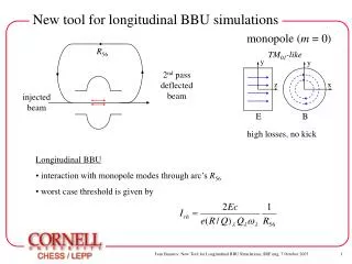
Run XI (meeting a beam line, w/ HOM couplers) HOM excitation (W) Vs frequency on a beam spectrum line for different QHOM max Vhom: 0.4MV I0=40mA I0=1% 0=0.1° fHOM=2113.2MHz HOM=100kHz QHOM=1E5 Vcav=0% cav=0° High HOM power has anyway to be handled 10 MeV 2.5°
Conclusions (personal draft – for discussion !) • In SPL-like linacs, BBU « out from the noise » can be damped: • N°1: lowering QHOM (e.g. using HOM couplers) This is the only solution for extreme conditions (100’s mA with high fluctuations, low HOM dispersion... ) or in circular machines (zero HOM frequency spread) OR • N°2: naturally Simply checking that HOM modes are sufficiently distributed from cavity to cavity (=100kHz seems even to be enough in the SPL case) • Simulating the SPL case without HOM couplers & with realistic input parameters shows apparently no longitudinal Beam Break Up instability rising • Cavities should be designed to avoid having a HOM mode exactly matching a beam resonance line.In the case where this is NOT achieved: • Without HOM couplers (high QHOM): very low probability to really hit the resonance, but could lead to a cavity quench + beam loss if it happens -> CURE = simply measure all cavities before installation to check • With HOM couplers (low QHOM): the probability to hit the resonance is far larger but not catastrophic -> HOM couplers have to be designed to evacuate large HOM powers continuously
Limits of these non-definitive conclusions... • Very poor statistics : more simulations should be performed • 10X pulses should be simulated to confirm the behavior with a « quasi-infinite » pulse train, and to check if any instability linked with the pulse structure is rising (even if for SPL, it is a priori non-relevant for such low pulsing frequencies) • The real SPL linac layout should be taken as input, including, for each cavity family, all HOM properties (f, Q, r/Q())... • More realistic (non-white) noises should be considered • Being aware that all this would imply enormous CPU time...