Download
1 / 36
360 likes | 555 Vues
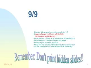
9/9. (today & thursday)correlation analysis; LSI (wed & Friday 10:30—11:45 BY210) dictionaries and indexing Homework 1 is due 9/16 (but will be collected 9/23) Homework 2 socket will open this week Project part A will be released

E N D
9/9 (today & thursday)correlation analysis; LSI (wed & Friday 10:30—11:45 BY210) dictionaries and indexing Homework 1 is due 9/16 (but will be collected 9/23) Homework 2 socket will open this week Project part A will be released Rao will not be around next week; however we can use the class time for reviews and such if needed. Remember: Don't print hidden slides!!
So many ways things can go wrong… Reasons that ideal effectiveness hard to achieve: • Document representation loses information. • Users’ inability to describe queries precisely. • Similarity function used not be good enough. • Importance/weight of a term in representing a document and query may be inaccurate • Same term may have multiple meanings and different terms may have similar meanings. Query expansion Relevance feedback LSI Co-occurrence analysis
Improving Vector Space Ranking • We will consider three techniques • Relevance feedback—which tries to improve the query quality Done. • Correlation analysis, which looks at correlations between keywords (and thus effectively computes a thesaurus based on the word occurrence in the documents) to do query elaboration • Principal Components Analysis (also called Latent Semantic Indexing) which subsumes correlation analysis and does dimensionality reduction.
Correlation/Co-occurrence analysis Co-occurrence analysis: • Terms that are related to terms in the original query may be added to the query. • Two terms are related if they have high co-occurrence in documents. Let n be the number of documents; n1 and n2 be # documents containing terms t1 and t2, m be the # documents having both t1 and t2 If t1 and t2 are independent If t1 and t2 are correlated Measure degree of correlation >> if Inversely correlated
Terms and Docs as mutually dependent vectors in In addition to doc-doc similarity, We can compute term-term distance Document vector Term vector • If terms are independent, the • T-T similarity matrix would • be diagonal • =If it is not diagonal, we can • use the correlations to add • related terms to the query • =But can also ask the question • “Are there independent • dimensions which define the • space where terms & docs are • vectors ?”
Association Clusters • Let Mij be the term-document matrix • For the full corpus (Global) • For the docs in the set of initial results (local) • (also sometimes, stems are used instead of terms) • Correlation matrix C = MMT (term-doc Xdoc-term = term-term) Un-normalized Association Matrix Normalized Association Matrix Nth-Association Cluster for a term tu is the set of terms tv such that Suv are the n largest values among Su1, Su2,….Suk
Example 11 4 6 4 34 11 6 11 26 Correlation Matrix d1d2d3d4d5d6d7 K1 2 1 0 2 1 1 0 K2 0 0 1 0 2 2 5 K3 1 0 3 0 4 0 0 Normalized Correlation Matrix 1.0 0.097 0.193 0.097 1.0 0.224 0.193 0.224 1.0 1thAssoc Cluster for K2is K3
Scalar clusters 200 docs with bush and iraq 200 docs with Iraq and saddam Is bush close to Saddam? Even if terms u and v have low correlations, they may be transitively correlated (e.g. a term w has high correlation with u and v). Consider the normalized association matrix S The “association vector” of term u Au is (Su1,Su2…Suk) To measure neighborhood-induced correlation between terms: Take the cosine-theta between the association vectors of terms u and v Nth-scalar Cluster for a term tu is the set of terms tv such that Suv are the n largest values among Su1, Su2,….Suk
Using Query Logs instead of Document Corpus • Correlation analysis can also be done based on query logs (i.e., the log of queries posed by the users). • Instead of doc-term matrix, you will start with query-term matrix • Query log correlation analysis has close parallels to the idea of collaborative filtering (the idea by which recommendation systems work..)
Example Normalized Correlation Matrix AK1 USER(43): (neighborhood normatrix) 0: (COSINE-METRIC (1.0 0.09756097 0.19354838) (1.0 0.09756097 0.19354838)) 0: returned 1.0 0: (COSINE-METRIC (1.0 0.09756097 0.19354838) (0.09756097 1.0 0.2244898)) 0: returned 0.22647195 0: (COSINE-METRIC (1.0 0.09756097 0.19354838) (0.19354838 0.2244898 1.0)) 0: returned 0.38323623 0: (COSINE-METRIC (0.09756097 1.0 0.2244898) (1.0 0.09756097 0.19354838)) 0: returned 0.22647195 0: (COSINE-METRIC (0.09756097 1.0 0.2244898) (0.09756097 1.0 0.2244898)) 0: returned 1.0 0: (COSINE-METRIC (0.09756097 1.0 0.2244898) (0.19354838 0.2244898 1.0)) 0: returned 0.43570948 0: (COSINE-METRIC (0.19354838 0.2244898 1.0) (1.0 0.09756097 0.19354838)) 0: returned 0.38323623 0: (COSINE-METRIC (0.19354838 0.2244898 1.0) (0.09756097 1.0 0.2244898)) 0: returned 0.43570948 0: (COSINE-METRIC (0.19354838 0.2244898 1.0) (0.19354838 0.2244898 1.0)) 0: returned 1.0 Scalar (neighborhood) Cluster Matrix 1.0 0.226 0.383 0.226 1.0 0.435 0.383 0.435 1.0 1thScalar Cluster for K2is still K3
On the database/statistics example database is most related to SQL and second most related to index Scalar Clusters t1= database t2=SQL t3=index t4=regression t5=likelihood t6=linear 1.0000 0.9604 0.8240 0.0847 0.1459 0.1136 0.9604 1.0000 0.9245 0.0388 0.1063 0.0660 0.8240 0.9245 1.0000 0.0465 0.1174 0.0655 0.0847 0.0388 0.0465 1.0000 0.8972 0.8459 0.1459 0.1063 0.1174 0.8972 1.0000 0.8946 0.1136 0.0660 0.0655 0.8459 0.8946 1.0000 Notice that index became much closer to database 3679 2391 1308 238 302 273 2391 1807 953 0 123 63 1308 953 536 32 87 27 238 0 32 3277 1584 1573 302 123 87 1584 972 887 273 63 27 1573 887 1423 Association Clusters 1.0000 0.7725 0.4499 0.0354 0.0694 0.0565 0.7725 1.0000 0.6856 0 0.0463 0.0199 0.4499 0.6856 1.0000 0.0085 0.0612 0.0140 0.0354 0 0.0085 1.0000 0.5944 0.5030 0.0694 0.0463 0.0612 0.5944 1.0000 0.5882 0.0565 0.0199 0.0140 0.5030 0.5882 1.0000
Beyond Correlation analysis: PCA/LSI • Suppose I start with documents described in terms of just two key words, u and v, but then • Add a bunch of new keywords (of the form 2u-3v; 4u-v etc), and give the new doc-term matrix to you. Will you be able to tell that the documents are really 2-dimensional (in that there are only two independent keywords)? • Suppose, in the above, I also add a bit of noise to each of the new terms (i.e. 2u-3v+noise; 4u-v+noise etc). Can you now discover that the documents are really 2-D? • Suppose further, I remove the original keywords, u and v, from the doc-term matrix, and give you only the new linearly dependent keywords. Can you now tell that the documents are 2-dimensional? • Notice that in this last case, the “true” dimensions of the data are not even present in the representation! You have to re-discover the true dimensions as linear combinations of the given dimensions. • Which means the current terms themselves are vectors in the original space.. added
PCA/LSI continued • The fact that keywords in the documents are not actually independent, and that they have synonymy and polysemy among them, often manifests itself as if some malicious oracle mixed up the data as above. • Need Dimensionality Reduction Techniques • If the keyword dependence is only linear (as above), a general polynomial complexity technique called Principal Components Analysis is able to do this dimensionality reduction • PCA applied to documents is called Latent Semantic Indexing • If the dependence is nonlinear, you need non-linear dimensionality reduction techniques (such as neural networks); much costlier.
Visual Example Data on Fish Length Height
Better if one axis accounts for most data variation What should we call the red axis? Size (“factor”)
Reduce Dimensions What if we only consider “size” We retain 1.75/2.00 x 100 (87.5%) of the original variation. Thus, by discarding the yellow axis we lose only 12.5% of the original information.
LSI as a special case of LDA • Dimensionality reduction (or feature selection) is typically done in the context of specific classification tasks • We want to pick dimensions (or features) that maximally differentiate across classes, while having minimal variance within any given class • When doing dimensionality reduction w.r.t a classification task, we need to focus on dimensions that • Increase variance across classes • and reduce variance within each class • Doing this is called LDA (linear discriminant analysis) • LSI—as given—is insensitive to any particular classification task and only focuses on data variance • LSI is a special case of LDA where each point defines its own class • This makes sense since “relevant” vs. “irrelevant” documents are query dependent In the example above, the Red line corresponds to the Dimension with most data variance However, the green line corresponds To the axis that does a better job of Capturing the class variance (assuming That the two different blobs correspond To the different classes)
9/11 In remembrance of all the lives and liberties lost to the wars by and on terror Guernica,Picasso
9/11Project Part A assignedWill send mail about tomorrow’s make-up class
Project A - Overview Create a search engine Vector Space Model Tf-Idf weights wij = tf(i,j) * idf(i) Cosine Similarity Sim(q,dj) = [ wij * wiq] / |dj| * |q| Hint: to improve performance, consider pre-computing |dj| for all documents rather than doing it each time you compute the similarity of a document
Project A – Lucene API Lucene - inverted index functionality Note: Use the version provided on the course website Useful Methods IndexReader Class terms() – returns the lexicon of terms in the index numDocs() – # of docs in the index docFreq(Term t) – # of docs containing term t termDocs(Term t) – returns docs containing term t termPositions(Term t) – returns docs containing term t along with the positions *optional*
Project A – Deliverables A write up explaining your algorithm and brief evaluation of its performance. Hardcopy showing the top 10 documents ranked by Vector Space model for the 10 example queries below. Hardcopy of your code with comments. Example Queries Fall semester Grades SRC Newsletter Decal Parking Hayden Library Transcripts Scholarship Admissions Demo
If you can do it for fish, why not to docs? • We have documents as vectors in the space of terms • We want to • “Transform” the axes so that the new axes are • “Orthonormal” (independent axes) • Notice that the new fish axes are uncorrelated.. • Can be ordered in terms of the amount of variation in the documents they capture • Pick top K dimensions (axes) in this ordering; and use these new K dimensions to do the vector-space similarity ranking • Why? • Can reduce noise • Can eliminate dependent variabales • Can capture synonymy and polysemy • How? • SVD (Singular Value Decomposition)
SVD is the Solution, but what is the problem? What we want to do: Given M of rank R, find a matrix M’ of rank R’ < R such that ||M-M’|| is the smallest Using multi-variable calculus, it can be shown that the solution is related to Eigen decomposition More specifically, Singular Value Decomposition, of a matrix SVD of a matrix dt is three matrices df, ff, tf such that M=df*ff*tf’ df is the eigen vectors of dt*dt’ tf is the eigen vectors of dt’*dt ff is a diagonal matrix whose diagonal values are the +ve square roots of eigen vectors of dt*dt’ or dt’*dt Rank of a matrix M is defined as the size of the largest square sub-matrix of M which has a non-zero determinant. The rank of a matrix M is also equal to the number of non-zero singular values it has Rank of M is related to the true dimensionality of M. If you add a bunch of rows to M that are linear combinations of the existing rows of M, the rank of the new matrix will still be the same as the rank of M. Distance between two equi-sized matrices M and M’; ||M-M’|| is defined as the sum of the squares of the differences between the corresponding entries (Sum (muv-m’uv)2) Will be equal to zero when M = M’
Bunch of Facts about SVD • Relation between SVD and Eigen value decomposition • Eigen value decomp is defined only for square matrices • Only square symmetric matrices have real-valued eigen values • PCA (principle component analysis) is normally done on correlation matriceswhich are square symmetric (think of d-d or t-t matrices). • SVD is defined for all matrices • Given a matrix dt, we consider the eigen decomposion of the correlation matrices d-d (dt*dt’) and tt (dt’*dt). SVD is • (a) the eigen vectors of d-d (2) positive square roots of eigen values of dd or tt (3)eigen vectors of tt • Both dd and tt are symmetric (they are correlation matrices) • They both will have the same eigen values • Unless M is symmetric, MMT and MTM are different • So, in general their eigen vectors will be different (although their eigen values are same) • Since SVD is defined in terms of the eigen values and vectors of the “Correlation matrices” of a matrix, the eigen values will always be real valued (even if the matrix M is not symmetric). • In general, the SVD decomposition of a matrix M equals its eigen decomposition only if M is both square and symmetric
Rank and Dimensionality What we want to do: Given M of rank R, find a matrix M’ of rank R’ < R such that ||M-M’|| is the smallest If you do a bit of calculus of variations, you will find that the solution is related to Eigen decomposition More specifically, Singular Value Decomposition, of a matrix Rank of a matrix M is defined as the size of the largest square sub-matrix of M which has a non-zero determinant. The rank of a matrix M is also equal to the number of non-zero singular values it has Rank of M is related to the true dimensionality of M. If you add a bunch of rows to M that are linear combinations of the existing rows of M, the rank of the new matrix will still be the same as the rank of M. Distance between two equi-sized matrices M and M’; ||M-M’|| is defined as the sum of the squares of the differences between the corresponding entries (Sum (muv-m’uv)2) Will be equal to zero when M = M’ • Suppose we did SVD on a doc-term matrix d-t, and took the top-k eigen values and reconstructed the matrix d-tk. We know • d-tk has rank k (since we zeroed out all the other eigen values when we reconstructed d-tk) • There is no k-rank matrix M such that ||d-t –M|| < ||d-t – d-tk|| • In other words d-tk is the best rank-k (dimension-k) approximation to d-t! • This is the guarantee given by SVD! Note that because the LSI dimensions are uncorrelated, finding the best k LSI dimensions is the same as sorting the dimensions in terms of their individual varianc (i.e., corresponding singualr values), and picking top-k
Overview of Latent Semantic Indexing Eigen Slide factor-factor (+ve sqrt of eigen values of d-t*d-t’or d-t’*d-t; both same) Doc-factor (eigen vectors of d-t*d-t’) (term-factor)T (eigen vectors of d-t’*d-t) Term Term dt df dfk dtk tft doc ff tfkt ffk Þ doc fxt dxt dxf fxf dxk kxk kxt dxt Reduce Dimensionality: Throw out low-order rows and columns Recreate Matrix: Multiply to produce approximate term- document matrix. dtk is a k-rank matrix That is closest to dt Singular Value Decomposition Convert doc-term matrix into 3matrices D-F, F-F, T-F Where DF*FF*TF’ gives the Original matrix back
New document coordinates d-f*f-f t1= database t2=SQL t3=index t4=regression t5=likelihood t6=linear F-F D-F 6 singular values (positive sqrt of eigen values of dd or tt) T-F Eigen vectors of dd (dt*dt’) (Principal document directions) Eigen vectors of tt (dt’*dt) (Principal term directions)
t1= database t2=SQL t3=index t4=regression t5=likelihood t6=linear For the database/regression example Suppose D1 is a new Doc containing “database” 50 times and D2 contains “SQL” 50 times
Visualizing the Loss 26 18 10 0 1 1 25 17 9 1 2 1 15 11 6 -1 0 0 7 5 3 0 0 0 44 31 17 0 2 1 2 0 0 19 10 11 1 -1 0 24 12 14 2 0 0 16 8 9 2 -1 0 39 20 22 4 2 1 20 11 12 Reconstruction (rounded) With 2 LSI dimensions Rank=2 Variance loss: 7.5% Rank=6 24 20 10 -1 2 3 32 10 7 1 0 1 12 15 7 -1 1 0 6 6 3 0 1 0 43 32 17 0 3 0 2 0 0 17 10 15 0 0 1 32 13 0 3 -1 0 20 8 1 0 1 0 37 21 26 7 -1 -1 15 10 22 Rank=4 Variance loss: 1.4% Reconstruction (rounded) With 4 LSI dimensions
LSI Ranking… • Given a query • Either add query also as a document in the D-T matrix and do the svd OR • Convert query vector (separately) to the LSI space • DFq*FF=q*TF • this is the weighted query document in LSI space • Reduce dimensionality as needed • Do the vector-space similarity in the LSI space
Using LSI Can be used on the entire corpus First compute the SVD of the entire corpus Store first k columns of the df*ff matrix [df*ff]k Keep the tf matrix handy When a new query q comes, take the k columns of q*tf Compute the vector similarity between [q*tf]k and all rows of [df*ff]k, rank the documents and return Can be used as a way of clustering the results returned by normal vector space ranking Take some top 50 or 100 of the documents returned by some ranking (e.g. vector ranking) Do LSI on these documents Take the first k columns of the resulting [df*ff] matrix Each row in this matrix is the representation of the original documents in the reduced space. Cluster the documents in this reduced space (We will talk about clustering later) MANJARA did this We will need fast SVD computation algorithms for this. MANJARA folks developed approximate algorithms for SVD
SVD Computation complexity • For an mxn matrix SVD computation is • O( km2n+k’n3) complexity • k=4 and k’=22 for best algorithms • Approximate algorithms that exploit the sparsity of M are available (and being developed)
Summary:What LSI can do • LSI analysis effectively does • Dimensionality reduction • Noise reduction • Exploitation of redundant data • Correlation analysis and Query expansion (with related words) • Any one of the individual effects can be achieved with simpler techniques (see scalar clustering etc). But LSI does all of them together.
LSI (dimensionality reduction) vs. Feature Selection • Before reducing dimensions, LSI first finds a new basis (coordinate axes) and then selects a subset of them • Good because the original axes may be too correlated to find top-k subspaces containing most variance • Bad because the new dimensions may not have any significance to the user • What are the two dimensions of the database example? • Something like 0.44*database+0.33*sql.. • An alternative is to select a subset of the original features themselves • Advantage is that the selected features are readily understandable by the users (to the extent they understood the original features). • Disadvantage is that as we saw in the Fish example, all the original dimensions may have about the same variance, while a (linear) combination of them might capture much more variation. • Another disadvantage is that since original features, unlike LSI features, may be correlated, finding the best subset of k features is not the same as sorting individual features in terms of the variance they capture and taking the top-K (as we could do with LSI)
LSI vs. Nonlinear dimensionality reduction • LSI only captures linear correlations • It cannot capture non-linear dependencies between original dimensions • E.g. if the data points are all falling on a simple manifold (e.g. a circle in the example below), • Then, the features are “non-linearly” correlated (here X2+Y2=c) • LSI analysis can’t reduce dimensionality here • One idea is to use techniques such as neural nets or manifold learning techniques • Another—simpler—idea is to consider first blowing up the dimensionality of the data by introducing new axes that are nonlinear combinations of existing ones (e.g. X2, Y2, sqrt(xy) etc.) • We can now capture linear correlations across these nonlinear dimensions by doing LSI in this enlarged space, and map the k important dimensions found back to original space. • So, in order to reduce dimensions, we first increase them (talk about crazy!) • A way of doing this implicitly is kernel trick.. Advanced; Optional