Mining Association Rules in Large Databases: Algorithms and Applications
Explore the concepts of association rule mining, frequent patterns, and correlations in databases. Learn about the Apriori algorithm for efficient rule discovery and pattern identification. Uncover the process of generating strong association rules from frequent itemsets and how to analyze support and confidence levels.

Mining Association Rules in Large Databases: Algorithms and Applications
E N D
Presentation Transcript
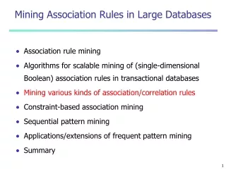
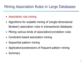
Mining Association Rules in Large Databases • Association rule mining • Algorithms for scalable mining of (single-dimensional Boolean) association rules in transactional databases • Mining various kinds of association/correlation rules • Constraint-based association mining • Sequential pattern mining • Applications/extensions of frequent pattern mining • Summary
What Is Association Mining? • Association rule mining: • A transaction T in a database supports an itemset S if S is contained in T • An itemset that has support above a certain threshold, called minimum support, is termed large (frequent) itemset • Frequent pattern: pattern (set of items, sequence, etc.) that occurs frequently in a database • Finding frequent patterns, associations, correlations, or causal structures among sets of items or objects in transaction databases, relational databases, and other information repositories.
What Is Association Mining? • Motivation: finding regularities in data • What products were often purchased together? — Beer and diapers • What are the subsequent purchases after buying a PC? • What kinds of DNA are sensitive to this new drug? • Can we automatically classify web documents?
Basic Concept: Association Rules • Let I={i1, i2, . . ., in} be the set of all distinct items • The association rules can be represented as “AB” where A and B are subsets, namely itemsets, of I • If A appears in one transaction, it is most likely that B also occurs in the same transaction
Basic Concept: Association Rules • For example • “BreadMilk” • “Beer Diaper” • The measurement of interestingness for association rules • support, s, probability that a transaction contains A∪B • s = support(“AB”) = P(A∪B) • confidence, c,conditional probability that a transaction having A also contains B. • c = confidence(“AB”) = P(B|A)
Customer buys both Customer buys diaper Customer buys beer Basic Concept: Association Rules • Let min_support = 50%, min_conf = 50%: • A C (50%, 66.7%) • C A (50%, 100%)
Basic Concepts: Frequent Patterns and Association Rules • Association rule mining is a two-step process: • Find all frequent itemsets • Generate strong association rules from the frequent itemsets • For every frequent itemset L, find all non-empty subsets of L. For every such subset A, output a rule of the form “A (L-A)” if the ratio of support(L) to support(A) is at least minimum confidence • The overall performance of mining association rules is determined by the first step
Mining Association Rules—an Example For rule AC: support = support({A}{C}) = 50% confidence = support({A}{C})/support({A}) = 66.6% Min. support 50% Min. confidence 50%
Mining Association Rules in Large Databases • Association rule mining • Algorithms for scalable mining of (single-dimensional Boolean) association rules in transactional databases • Mining various kinds of association/correlation rules • Constraint-based association mining • Sequential pattern mining • Applications/extensions of frequent pattern mining • Summary
The Apriori Algorithm • The name, Apriori, is based on the fact that the algorithm uses prior knowledge of frequent itemset properties • Apriori employs an iterative approach known as a level-wise search, where k-itemsets are used to explore (k+1)-itemsets • The first pass determines the frequent 1-itemsets denoted L1 • A subsequence pass k consists of two phases • First, the frequent itemsets Lk-1 are used to generate the candidate itemsets Ck • Next, the database is scanned and the support of candidates in Ck is counted • The frequent itemsets Lk are determined
Apriori Property • Apriori property: any subset of a large itemset must be large • If {beer, diaper, nuts} is frequent, so is {beer, diaper} • Every transaction having {beer, diaper, nuts} also contains {beer, diaper} • Anti-monotone: if a set cannot pass a test, all of its supersets will fail the same test as well
Apriori: A Candidate Generation-and-test Approach • Apriori pruning principle: If there is any itemset which is infrequent, its superset should not be generated/tested! • Method: join and prune steps • Generate candidate (k+1)-itemsets Ck+1 from frequent k-itemsets Lk • If any k-subset of a candidate (k+1)-itemset is not in Lk, then the candidate cannot be frequent either and so can be removed from Ck • Test the candidates against DB to obtain Lk+1
The Apriori Algorithm—Example • Let the minimum support be 20%
The Apriori Algorithm • Pseudo-code: Ck: Candidate itemset of size k Lk : frequent itemset of size k L1 = {frequent items}; for(k = 1; Lk !=; k++) Ck+1 = candidates generated from Lk; for each transaction t in database increment the count of all candidates in Ck+1 that are contained in t end Lk+1 = candidates in Ck+1 with min_support end returnkLk;
Important Details of Apriori • How to generate candidates? • Step 1: self-joining Lk • Step 2: pruning • How to count supports of candidates? • Example of candidate-generation • L3={abc, abd, acd, ace, bcd} • Self-joining: L3*L3 • abcd from abc and abd • acde from acd and ace • Pruning: • acde is removed because ade is not in L3 • C4={abcd}
How to Generate Candidates? • Suppose the items in Lk-1 are listed in an order • Step 1: self-joining Lk-1 insert intoCk select p.item1, p.item2, …, p.itemk-1, q.itemk-1 from Lk-1 p, Lk-1 q where p.item1=q.item1, …, p.itemk-2=q.itemk-2, p.itemk-1 < q.itemk-1 • Step 2: pruning forall itemsets c in Ckdo forall (k-1)-subsets s of c do if (s is not in Lk-1) then delete c from Ck
Challenges of Frequent Pattern Mining • Challenges • Multiple scans of transaction database • Huge number of candidates • Tedious workload of support counting for candidates • Improving Apriori: general ideas • Reduce passes of transaction database scans • Shrink number of candidates • Facilitate support counting of candidates
DIC — Reduce Number of Scans • The intuition behind DIC is that it works like a train running over the data with stops at intervals Mtransactions apart. • If we consider Apriori in this metaphor, all itemsets must get on at the start of a pass and get off at the end. The 1-itemsets take the fist pass, the 2-itemsets take the second pass, and so on. • In DIC, we have the added flexibility of allowing itemsets to get on at any stop as long as they get off at the same stop the next time the train goes around. • We can start counting an itemset as soon as we suspect it may be necessary to count it instead of waiting until the end of the previous pass.
DIC — Reduce Number of Scans • For example, if we are mining 40,000 transactions and M = 10,000, we will count all the l-itemsets in the first 40,000 transactions we will read. However, we will begin counting 2-itemsets after the first 10,000 transactions have been read. We will begin counting 3-itemsets after 20,000 transactions. • We assume there are no 4-itemsets we need to count. Once we get to the end of the file, we will stop counting the l-itemsets and go back to the start of the file to count the 2 and 3-itemsets. After the first 10,000 transactions, we will finish counting the 2-itemsets and after 20,000 transactions, we will finish counting the 3-itemsets. In total, we have made 1.5 passes over the data instead of the 3 passes a level-wise algorithm would make.
DIC — Reduce Number of Scans • DIC addresses the high-level issues of when to count which itemsets and is a substantial speedup over Apriori, particularly when Apriori requires many passes.
Once both A and D are determined frequent, the counting of AD begins Once all length-2 subsets of BCD are determined frequent, the counting of BCD begins DIC — Reduce Number of Scans ABCD ABC ABD ACD BCD AB AC BC AD BD CD Transactions 1-itemsets B C D A 2-itemsets Apriori … {} Itemset lattice 1-itemsets 2-items DIC 3-items
DIC — Reduce Number of Scans • Solid box - confirmed large itemset - an itemset we have finished counting that exceeds the support threshold. • Solid circle - confirmed small itemset - an itemset we have finished counting that is below the support threshold. • Dashed box - suspected large itemset - an itemset we are still counting that exceeds the support threshold. • Dashed circle - suspected small itemset - an itemset we are still counting that is below the support threshold.
DIC Algorithm • The DIC algorithm works as follows: • The empty itemset is marked with a solid box. All the l-itemsets are marked with dashed circles. All other itemsets are unmarked.
DIC Algorithm • The DIC algorithm works as follows: • Read M transactions. We experimented with values of Mranging from 100 to 10,000. For each transaction, increment the respective counters for the itemsets marked with dashes. • If a dashed circle has a count that exceeds the support threshold, turn it into a dashed square. If any immediate superset of it has all of its subsets as solid or dashed squares, add a new counter for it and make it a dashed circle.
DIC Algorithm • The DIC algorithm works as follows: • If a dashed itemset has been countedthrough all the transactions, make it solid and stop counting it. • If we are at the end of the transaction file, rewind to the beginning. • If any dashed itemsets remain, go to step 2.
DIC Summary • There are a number of benefits to DIC. The main one is performance. If the data is fairly homogeneous throughout the file and the interval M is reasonably small, this algorithm generally makes on the order of two passes. This makes the algorithm considerably faster than Apriori which must make as many passes as the maximum size of a candidate itemset. • Besides performance, DIC provides considerable flexibility by having the ability to add and delete counted itemsets on the fly. As a result, DIC can be extended to incremental update version.
Partition: Scan Database Only Twice • Any itemset that is potentially frequent in DB must be frequent in at least one of the partitions of DB • Scan 1: partition database and find local frequent patterns • Scan 2: consolidate global frequent patterns
Partition Algorithm Algorithm Partition: 1) P = partition_database(D) 2) n = Number of partitions 3) for i=1 to n begin // Phase I 4) read_in_partition(piP) 5) Li = gen_large_itemsets(pi) 6) end 7) for (i=2; ≠, j=1, 2, …, n; i++) do 8) = ∪j=1,2,…,n // Merge Phase 9) for i=1 to n begin // Phase II 10) read_in_partition(piP) 11) for all candidates cCG gen_count(c, pi) 12) end 13) LG = {cCG | c.count min_sup}
Partition Algorithm Procedure gen_large_itemsets() 1) = {large 1-itemsets along with their tidlists} 2) for (k=2; ≠; k++) do begin 3) forall itemsets l1 do begin 4) forall itemsets l2 do begin 5) ifl1[1]=l2[1] ^ l1[2]=l2[2] ^ … ^ l1[k-2]=l2[k-2] ^ l1[k-1]<l2[k-1] then 6) c = l1[1].l1[2]...l1[k-1].l2[k-1] 7) ifc cannot be pruned then 8) c.tidlist = l1.tidlist∩l2.tidlist 9) if (|c.tidlist| / |p|) min_supthen 10) = ∪{c} 11) end 12) end 13) end 14) return ∪k
Sampling for Frequent Patterns • Select a sample of original database, mine frequent patterns within sample using Apriori • Scan database once to verify frequent itemsets found in sample, only bordersof closure of frequent patterns are checked • Example: check abcd instead of ab, ac, …, etc. • Scan database again to find missed frequent patterns
Sampling Algorithm Algorithm Sampling (Phase I): 1) draw a random sample s from D; 2) compute S with lowered minimum support threshold; 3) compute F = {X|XS∪Bd-(S), xX, x.countmin_sup}; 4) output all X; 5) report if there possibly was a failure;
Sampling Algorithm Algorithm Sampling (Phase II): 1) repeat 2) compute S = S∪Bd-(S); 3) until S does not grow; 4) compute F = {X|XS, xX, x.count min_sup}; 5) output all X;
DHP (Direct Hashing and Pruning): Reduce the Number of Candidates • A k-itemset whose corresponding hashing bucket count is below the threshold cannot be frequent
Bottleneck of Frequent-pattern Mining • Multiple database scans are costly • Mining long patterns needs many passes of scanning and generates lots of candidates • To find frequent itemset i1i2…i100 • # of scans: 100 • # of Candidates: (1001) + (1002) + … + (100100) = 2100-1 = 1.27*1030 ! • Bottleneck: candidate-generation-and-test • Can we avoid candidate generation?