Download

1 / 54
540 likes | 778 Vues
EC120 TEST #1 EXAM-AID. Tutor: Jason “J-Dawg” Frittaion Coordinator: Alanna Davoren Some images used from course slides. AGENDA. Go through Chapters 1-6 Intro to Economics and Opportunity Cost PPF, Trade, and Comparative Advantage Demand, Supply, and Price Elasticity

E N D
EC120 TEST #1 EXAM-AID Tutor: Jason “J-Dawg” Frittaion Coordinator: Alanna Davoren Some images used from course slides.
AGENDA Go through Chapters 1-6 • Intro to Economics and Opportunity Cost • PPF, Trade, and Comparative Advantage • Demand, Supply, and Price • Elasticity • Government Policy (Price Floors and Ceilings)
A Few Qualitative Points • Economics is pretty much the study of motives and relationships that cause all the interactions of the market. • The economy is self-organizing through these motives (self-interest, incentives, etc.). When the economy is self-organizing, we consider it to be an open market (constantly striving for efficiency). • Land, labour, and capital are what produce the goods and services we consume (also known as factors of production). • These resources are however limited (scarcity). Therefore we must manage these resources, making decisions among our needs and unlimited wants. • Opportunity cost illustrates this concept of trade-off.
Opportunity Cost “The foregone benefits of the next best alternative.” These costs include explicit costs (out of pocket expenses such as paying for a movie ticket) and implicit costs (foregone earnings such as going to the movies versus working that night) They DO NOT include sunk costs (unrecoverable costs). These are basically the costs that must be incurred regardless of which course of action is taken.
EXAMPLE # 1 Answer: (b) WHY?If he hires a plumber and chooses to go to work, he will have to pay the plumber $200, which is an out of pocket expense; hence it will be included as an opportunity cost. If he does it himself, his foregone earnings that he could’ve made by working would be his opportunity cost.
EXAMPLE # 2 Answer: (b) WHY?Before the fertilizer was discovered, if the farmer had chosen to plant potatoes (5), he would have to give up the benefit of growing 10 corn. In other words, in order to grow 1 potato, he would have to give up 2 corn. Now that a new fertilizer has been discovered which doubles the per acre yield, in order to grow potatoes (10), he would have to give up the benefit of growing 20 corn. In other words, in order to grow 1 potato, you would have to give up 2 corn again. Same rule applies to the option of growing corn instead.
Production Possibilities Frontier • Shows the combinations of goods that can be produced if all resources are fully employed. • Points inside the PPF are attainable, but you are not fully using your resources. • Points outside are unattainable and can only be attained by new technology or a stronger labour force. • Slope of the PPF indicates opportunity cost of the good on the x-axis. • PPF has a concave shape because OC rises as productivity declines in the transfer of resources. • PPF shifts if technology or resources change. • It can also pivot on one axis if technology or resources only changes for one good.
Production Possibility Frontier The negatively sloped boundary shows the combinations that are just attainable when all of society’s resources are efficiently employed.
Trade • Adam Smith proposed trade in terms of absolute cost. • David Ricardo took it a step further saying that trade should be based on a comparative level (comparing opportunity costs to other countries). • By trading, goods can be acquired at lower opportunity costs and specialization can further increase consumption possibilities. • The terms of trade between two countries (what to price the goods at in terms of the other goods, I.e. 1 pencil sharpener = 3 cans of pop) have to be so that each country is never paying more than the opportunity cost of producing the good domestically.
Comparative Advantage “The situation that exists when a country can produce a good with less foregone output of other goods than can another country.” • Comparative advantages reflect opportunity costs that differ between countries. • Even though a country may have an absolute advantage in all goods, it cannothave a comparative advantage in all goods. • The gains from specialization and trade depend on the pattern of comparative, not absolute advantage. • Absolute advantage refers to when a country can produce more of a good, given the same amount of resources (usually referring to labour).
Gains from Trade • Trade allows importing countries to acquire goods at a lower opportunity cost than if they produced the goods themselves. • Whenever opportunity costs differ between countries, it is always possible to increase consumption of goods if countries specialize in producing the product they have a comparative advantage in. • TIP: Whenever calculating OC, put the one you want to find in the bottom (denominator). • I.e. with guns and pillows. If I want to find the OC of guns in Canada, do: Canadian Pillows Canadian Guns
Example! Answer: b) Why? Overall, the Foreign cannot produce more of either good (no absolute advantage), but it’s opportunity cost is lower when it comes to pillows.
Example! Answer: b) Remember, no country would ever want to trade when the relative price of a good is greater than it’s opportunity cost for that good (because they may as well make it themselves then). The OC of guns ranges between 2-2.5. Therefore, terms of trade must be within this range.
Example! • Answer: b) • Wrong – why would countries export goods just to import the same two goods back? • Correct – the Foreign country has the comparative advantage and should therefore export (as opportunity cost is lower). • Wrong – the Home country has a higher (opportunity) cost of making pillows, so they should leave it to the Foreign country. • Wrong – the Home country has a comparative advantage in making guns. • Wrong – both can gain from trade by specializing in the good which they have lower opportunity cost in.
Supply and Demand Quantity Demanded:total amount of any particular good or service that consumers wish to purchase in some time period at a certain price. Quantity Supplied: total amount of any particular good or service that suppliers wish to supply in some time period at a certain price. Price Demand Pe Supply Qe Quantity
Factors of Demand • Change in the price of a substitute good • Direct relationship (I.e. Pepsi prices increases, Coke Demand increases) • Change in the price of a complementary good • Inverse relationship (I.e. Pillow prices rise, pillowcase demand falls) • Change in consumer income • Direct relationship (I.e. minimum wage increases, demand for beer increases) • Change in population • Direct relationship (every fall, the population of Waterloo increases by about 30,000 students, demand for eating out increases) • Change in tastes and Preferences • Direct Relationship (The people of Waterloo generally become more health conscious, the demand for healthy food increases) • Future expectations • Direct Relationship (Y2K example: the public thinks some crazy stuff is gonna go down, therefore the demand for canned soup sky rockets now )
Factors of Supply • Price of an input • Inverse Relationship: the price of yarn goes up, therefore the supply of J-Dawg’s hand knitted mittens goes down • Technology • Direct relationship: new technology is discovered in regards to getting the caramel inside of the chocolate, therefore the supply of Caramilk bars goes up • # of Suppliers • Direct relationship: the number of restaurants being built in Waterloo goes up, therefore the supply increases • Expectations • If suppliers expect prices to rise in the future, they may reduce supply in order to sell more later at a higher price • Natural Events • Weather that destroys crops, or a severe tornado that destroys machinery and a factory will decrease the supply of that good.
Demand and Supply Key Points TO KEEP IN MIND: • Both quantity demanded and quantity supplied represent flows of those goods over a time period (not a stock of goods). • For the time being, we are assuming markets to be perfectly competitive (many buyers and sellers who have no appreciable influence over prices – the market determines prices). Therefore, market forces cause price to always move towards EQUILIBRIUM (where Qd = Qs). • A change in a good’s price (P) causes a • Movement along a demand or supply curve and a change in quantity demanded or supplied • A change in any of the factors of demand or supply (Price not being one of them) causes • Shiftof a demand/supply curve
Example! • Answer: a) • Correct – Wages of workers are an input, price of an input going up causes supply to decrease. • Wrong – This is a factor of demand. • Wrong – An increase in the number of suppliers will increase the supply. • Wrong – A decrease in the price causes a decrease in the quantity supplied, not the actual supply. • Wrong – Wrong because d) is wrong.
Four Laws of Demand and Supply • An increase in demand causes an increase in both the equilibrium price and the equilibrium quantity exchanged. • A decrease in demand causes a decrease in both the equilibrium price and quantity exchanged. (when demand shifts, P and Q move in the same direction!)
Four Laws of Demand and Supply Continued…. 3. An increase in supply causes adecreasein the equilibrium price and an increase the equilibrium quantity exchanged. 4. A decrease in supply causes an increasethe equilibrium priceand a decreasequantity exchanged. (when Supply shifts, P and Q move in opposite directions!)
Laws Sum Up If… • D Pe Qe • D Pe Qe • S Pe Qe • S Pe Qe
Are there any questions up to this point?! A Short Commercial Break (?)
Price Elasticity of Demand The price elasticity of demand is the measure of responsiveness of quantity of a product demanded to a change in that product’s price. Percentage changes are measured using the average price and quantity so that η is the same for a price rise or a price fall.
ηalong a Linear Demand Curve A linear demand has a constant slope but a non-constant elasticity.
Elasticity of Demand • Inelastic Demand: a situation in which, for a given percentage change in price, there is a smaller percentage change in quantity demanded; elasticity is less than one. • Ex: Pace Maker, certain drugs… • In general, the steeper a demand curve is, the more inelastic it is (consumers are less responsive to price changes). • Elastic Demand: the situation in which for a given percentage change in price there is a greater percentage change in quantity demanded. • Ex: blue ink pen • In general, the flatter a demand curve is, the more elastic it is (consumers are more responsive to price changes). These same concepts can be applied to supply curves.
Determinants of η • ηdepends on the ability and willingness of buyers to substitute between products. • ηis higher.. • In long-run than in the short-run • If you give buyers more time, individuals will substitute away – hence higher elasticity • The more narrowly defined a good is (I.e. Pepsi is more elastic than pop in general). • Smaller categories have more substitutes – hence higher elasticity • The larger the share of a consumer’s budget it represents (I.e. 20% change in car prices vs. 20% change in coffee prices)
Elasticity and Consumer Spending • Consumer Spending = P x QD • If demand is elastic then.. • Pand consumer spending are inversely related • If demand is inelastic then.. • P and consumer spending are directly related • If demand is unit elastic then.. • Spending is unaffected by price changes
Example! • If demand is inelastic then will a drought result in higher(increased spending) or lower(decreased spending) revenues for sellers collectively?
Decrease in Supply and Total Expenditure With a decrease in supply S2 is still considered in the inelastic portion of the demand curve (S1 to S2) and thus total expenditure will increase (price is increasing, spending increases). With a larger decrease in supply, that overshoots the equilibrium past the point of unit-elasticity, the supply curve intersects the elastic portion of the demand curve whereby price increases but total expenditure begins to decrease. Making it possible for total expenditure from S1 to S3 to decrease (or increase if not overshot by too much). P S3 S 2 S 1 Elastic Demand Inelastic Demand Q Q3 Q2 Q1
More Elasticity Problems What is the elasticity in the following cases: • As the price of CDs fell, product revenue rose. P decreased, Revenue(spending) increased –> when P and total consumer spending are inversely related, we know that the demand is price ELASTIC • I gotta have coffee no matter what the price Gotta have it –> INELASTIC (prices go up but people don’t stop buying -> price and total spending move up together. • I spend $50/day on gas regardless of the price Spending stays constant – hence UNIT ELASTIC
Price Elasticity of Supply ηs= % change in quantity supplied % change in price Determinants of ηs: ηs is higher.. • in the long-run than in the short run • If inputs can be easily re-allocated • I.e. the easier a farmer can switch between growing wheat and corn, the more responsive they will be to changes in wheat or corn prices. So if wheat prices drop, they switch to corn and reduce wheat supply.
Cross Price Elasticity of Demand ηxy = % change in quantity demanded of good x % change in price of good y ηxy > 0 if x and y are substitutes (coke/pepsi) ηxy < 0 if x and y are complements (gas/car)
Income Elasticity of Demand ηY= % change in quantity demanded of good x % change in income ηY > 0 for normal goods income increases, demand increases if 0 < ηY < 1, the good is said to be a necessity if ηY > 1, the good is said to be a luxury ηY < 0 for inferior goods income increase, demand decreases
Example! • Coffee is a normal good. A decrease in income will • Increase the equilibrium price of coffee and increase the equilibrium quantity of coffee • Increase the equilibrium price of coffee and decrease the equilibrium quantity of coffee • Decrease the equilibrium price of coffee and decrease the equilibrium quantity of coffee • Decrease the equilibrium price of coffee and increase the quantity supplied of coffee • Cause none of the above • ANSWER: c) • The definition of a normal good is that with income increases, the demand for that good also increases. The same pattern is applied when income decreases. Decreased income decreases the demand for coffee (resulting in a leftward shift of D). The shift in the demand curve causes equilibrium price and quantity to move in same direction. So it’s a) or c). We know income directly relates to demand for normal goods, therefore P and Q decrease along with it.
Example! • If turnips are an inferior good, then ceteris paribus, an increase in the price of turnips will cause • A decrease in the demand for turnips • An increase in the demand for turnips • A decrease in the supply of turnips • An increase in the supply of turnips • None of the above ANSWER: e) This question attempts to trick students. Any change in the price of a good is already taken into account by your graph (Price is on the y axis). The demand and supply curves formed represent all the quantities demanded and supplied at each price (so a change in one is just a movement along the already existing curves).
Adding in Tax • Governments may come into the open market and charge an excise (or commodity) tax on specific goods. • If they legislate the tax to be paid by the consumers, consumers are still only willing to pay as much for the good as they did before. • But we need to find the quantity and price where consumers are paying the minimum amount that suppliers are willing to sell for (and the sellers aren’t receiving any of the tax money consumers are paying). P(Consumer) = P(Seller) + Tax • So, we shift the demand curve inward to the left to include tax to find our equilibrium quantity. • Meanwhile, if the tax is legislated so that suppliers pay it directly, the same interactions happen on the supply side and we end up shifting the supply curve upward and to the left to find equilibrium quantity.
Tax Paid by Buyers or Sellers • EITHER WAY: Charging buyers or sellers, will cause equilibrium quantity to decrease. Pretty much, who we charge doesn’t make a difference. The burden of the tax will depend on who is less responsive to the tax change.
The Burden • The total tax revenue collected by the government is equal to the tax (difference between price paid by consumers and collected by sellers) multiplied by the quantity (with tax) sold. • Tax rev = [(PDT – PST)*QET] • To assess who takes on how much of this tax burden, we measure the total paid per group: • For consumers, the increase in price multiplied by the quantity (with tax) sold. Consumer Burden = [(PDT - PENoTax)*(QET)] • For suppliers, the decrease in the price they receive multiplied by the quantity (with tax) sold. Supplier Burden = [(PENotax – PST)*(QET)]
General Rules About the Burden • Whichever side (Demand or Supply/Buyers or Sellers) is more inelastic (more steep slope), bares the greater burden of the tax as they are the least responsive to the price change. • The more elastic (less steep, flatter slope) between the buyers and the sellers are the ones who will bare the least of the burden.
Example! Answer: a) Since the consumers have a higher elasticity than the producers, the producers are less responsive to the change and end up paying more of the tax. Because consumers aren’t perfectly elastic, they will still end up taking on some of the tax burden.
Price Floor • A price floor is a minimum permissible price(ex. minimum wage) • An effective price floor.. • Is set abovethe equilibrium price • Results in fewerunits being sold • Makes buyers worse off, some sellers better off & other sellers worse off • Causes excess supply