Control Flow Analysis
Control Flow Analysis. Compiler Baojian Hua bjhua@ustc.edu.cn. Front End. lexical analyzer. source code. tokens. abstract syntax tree. parser. semantic analyzer. IR. Middle End. translation. AST. IR1. translation. IR2. other IR and translation. asm. Intermediate Representation.


Control Flow Analysis
E N D
Presentation Transcript
Control Flow Analysis Compiler Baojian Hua bjhua@ustc.edu.cn
Front End lexical analyzer source code tokens abstract syntax tree parser semantic analyzer IR
Middle End translation AST IR1 translation IR2 other IR and translation asm
Intermediate Representation • Trees and Dags • high-level, program structures • 3-address code • low-level, closer to ISA • Today, control-flow graph (CFG) • more refined 3-address code • good for optimizations
3-address Code: Recap if (x < y){ z = 4; m = 3; } else{ z = 6; m = 5; } Cjmp (x<y, L_1, L_2); L_1: z = 4; m = 3; jmp L_3; L_2: z = 6; m = 5; jmp L_3; L_3:
Control Structure Cjmp (x<y, L_1, L_2); L_1: z = 4; m = 3; jmp L_3; L_2: z = 6; m = 5; jmp L_3; L_3: Cjmp (x<y, L_1, L_2); L_2 L_1 z = 4; m = 3; jmp L_3; z = 6; m = 5; jmp L_3; L_3 …;
Moral • This graph-based representation is good for many purposes: • flow analysis: • for many program analysis, the program internal structure is important • enable other analysis: • such as data-flow analysis (to be discussed later) • scheduling: • try to minimizing “jump”s by rearranging the program structures
Basic Blocks & Control Flow Graph • A basic block is a sequence of basic statements, executing from the beginning and exiting at the end • can NOT enter the middle • can NOT exit the from the middle • no interleaving “jump” or “branch” • Control-flow graph is a graph consisting of basic blocks as vertices
Basic blocks and CFG Cjmp (x<y, L_1, L_2); block label (name) L_2 L_1 z = 4; m = 3; jmp L_3; z = 6; m = 5; jmp L_3; basic blocks ending with a “jump” statement edge stands for control transfer L_3 …;
Control Flow GraphData Structure // Just a refined 3-address code s -> x = v1 + v2 | x = v | x = f (v1, v2, …, vn) j -> Jump L | Cjump (v, L1, L2) | return b -> Label L; s1; s2; …, sn j; f -> b1, …, bn prog -> f1, …, fn
Conversion into CFG • One can start directly from AST or HIL: • good for language like MiniJava, which has regular control structures • Or one can start from 3-adress code or other IRs: • may be easier for languages such as C, which have unstructured controls (e.g., goto) • Next, we discuss techniques dealing with CFG
CFG Traversal • Standard graph traversal algorithms: • DFS, BFS, … • Important for linearization of nodes: • Topo-sort order, quasi-topo-sort order, and reverse top-sort order • We leave these operations to your algorithm course, and next we discuss two applications: • dead-code eliminations (optimizations) • extended basic blocks (EBBs)
#1: Dead code (block) elimination example int f () { int i = 3; while (i<10){ i = i+1; printi(i); continue; printi(i); } return 0; } L0 i=3 i<10? L1: L2 L1 printi(i) jump L0 L3 printi(i) jump L2 L2 return 0
#1: Dead code (block) elimination algorithm // algorithm // input: a CFG g for f // output: a new CFG for // function f dfs (g); for (each node n in g) if (!visited(n)) delete (n); L0 i=3 i<10? L1: L2 L1 printi(i) jump L0 L3 printi(i) jump L2 L2 return 0
#2: Extended basic blocks • Extended blocks from a block A is a maximal set of blocks with no join • that is, every block (except for A) should have just one predecessor • e.g., in the following graph, extended blocks from A are {A, B, C} A C B D
#2: EBBs A // Algorithm: give a node n, // calculate EBB for this node. // This is just a variant // of DFS ebb = {}; build_ebb (n: node) ebb \/= {n}; foreach (successor m of n) if (|pred(m)| ==1 && m\not\in ebb) build_ebb (m); C B D
Dominators • A node a dominates a node d, iff every path from the entry node s0 to the node d goes through the node a • a is a dominator of node d • every node dominates itself • Dominator relationship is a partial order • that is: reflexive, anti-symmetry, transitive • leave the proof to you!
Example 1 A node a dominates a node d, iff every path from the entry node s0 to the node d goes through the node a. We write it as: a dom d 2 3 4 D[6] D[5] 1 dom 2 2 dom 4 5 6 2 dom 7 8 7 D[7] 4 dom 7 9 6 dom 7 ??? 11 D[n]={all nodes x | x dom n} 10 12
Equation • Fix-point algorithm • Can be accelerated by first ordering the nodes • quasi-topo sort order • Or by Tarjan’s algorithm (nearly linear time)
Step #1: initialization D[s0]={s0} D[n]={all nodes} D[1]={1} 1 D[2]={1, …, 12} 2 3 4 D[4]={1, …, 12} D[3]={1, …, 12} D[5]={1, …, 12} 5 6 D[6]={1, …, 12} D[8]={1, …, 12} 8 7 D[7]={1, …, 12} 9 D[9]={1, …, 12} 11 D[11]={1, …, 12} D[10]={1, …, 12} 10 12 D[12]={1, …, 12}
Step #2: calculate a quasi-topo sort order quasi top-sort order: 1, 2, 3, 4, 5, 8, 9, 10, 6, 7, 11, 12 D[1]={1} 1 D[2]={1, …, 12} 2 3 4 D[4]={1, …, 12} D[3]={1, …, 12} D[5]={1, …, 12} D[6]={1, …, 12} 5 6 D[8]={1, …, 12} 8 7 D[7]={1, …, 12} 9 D[9]={1, …, 12} 11 D[11]={1, …, 12} D[10]={1, …, 12} 10 12 D[12]={1, …, 12}
Step #3: calculate fix-point quasi top-sort order: 1, 2, 3, 4, 5, 8, 9, 10, 6, 7, 11, 12 D[1]={1} 1 {1, 2} D[2]={1, …, 12} 2 {1, 2, 4} {1, 2, 3} 3 4 D[4]={1, …, 12} D[3]={1, …, 12} {1, 2, 4, 5} {1, 2, 4, 6} D[5]={1, …, 12} 5 6 D[6]={1, …, 12} {1, 2, 4, 5, 8} D[8]={1, …, 12} {1, 2, 4, 7} 8 7 D[7]={1, …, 12} {1, 2, 4, 5, 8, 9} {1, 2, 4, 7, 11} 9 D[9]={1, …, 12} 11 D[11]={1, …, 12} {1, 2, 4, 5, 8, 9, 10} {1, 2, 4, 12} D[10]={1, …, 12} 10 12 D[12]={1, …, 12}
Step #3: calculate fix-point quasi top-sort order: 1, 2, 3, 4, 5, 8, 9, 10, 6, 7, 11, 12 D[1]={1} 1 D[2]={1, 2} 2 3 4 D[4]={1, 2, 4} D[3]={1, 2, 3} D[5]={1,2,4,5} 5 6 D[6]={1, 2, 4, 6} D[8]={1,2,4,5,8} 8 7 D[7]={1, 2, 4, 7} 9 D[9]={1,2,4,5,8,9} 11 D[11]={1,2,4,7,11} D[10]={1,2,4,5,8,9,10} 10 12 D[12]={1, 2, 4, 12}
Immediate dominator • Intuitively, an immediate dominatorx for a node n is a node that is most close to n • x dom n, x!=n • for any y dom n, then y dom x • One can prove a theorem stating that for every node n (except for s0), n has just one immediate dominator • write n’s immediate dominator as idom(n)
Immediate dominator quasi top-sort order: 1, 2, 3, 4, 5, 8, 9, 10, 6, 7, 11, 12 D[1]={1} 1 D[2]={1, 2} 2 3 4 D[4]={1, 2, 4} D[3]={1, 2, 3} D[5]={1,2,4,5} 5 6 D[6]={1, 2, 4, 6} D[8]={1,2,4,5,8} 8 7 D[7]={1, 2, 4, 7} 9 D[9]={1,2,4,5,8,9} 11 D[11]={1,2,4,7,11} D[10]={1,2,4,5,8,9,10} 10 12 D[12]={1, 2, 4, 12}
Dominator Tree 1 2 3 4 5 6 7 12 8 11 9 10
Dominator Calculation Revisited • In 2005, Cooper et. al, published an interesting paper • dominator tree-based, easy to implement • Even comparable with Tarjan’s algorithm • Lesson: careful engineering of well-known slow algorithm may be profitable
Strict dominator • Node x is a strict dominator of y, if x dominates y, and x<>y • sdom (x) = dom(x)-{x} • Dominance frontier of a node x: • a set of nodes y such that x dominates a predecessor p of node y, but does not strictly dominates y • df(x)=? • read the algorithm in Tiger 19.1
Intuition for Dominance Frontier s0 x p s q t
Dominance Frontier Walk the dominator tree in post-order: 3, 10, 9, 8, 5, 6, 11, 7, 12, 4, 2, 1 1 1 df(1)={} df(2)={2} 2 2 df(4)={2} 3 4 3 4 df(3)={2} df(6)={7} 5 6 5 df(5)={5, 12, 7} 6 12 7 df(12)={} 8 8 7 df(7)={12} df(8)={5, 12, 8} 9 9 11 11 df(11)={12} df(9)={5, 12, 8} 10 10 12 df(10)={5, 12}
Natural Loops • Given a back edge m->h (for dominance), the natural loop for m->h is all nodes x that dominated by h and can reach m without going through h
Loops(3->2)={2, 3} Loops(4->2)={2, 4} Loops(10->5)={5,8,9,10} Loops(9->8)={8, 9} Natural Loops 1 1 2 2 3 4 3 4 5 6 5 6 12 7 8 8 7 9 9 11 11 10 10 12
Motivation Node 1 controls whether or not node 2 will execute. We say node 2 is control-dependent on node 1. 1 A[0] = 0 1 2 A[1] = 1 2 3 3 Suppose we are running this program on a two-core CPU with core C0, C1. Then can we run node 1 on C0 and node2 on C1? (Parallelization!) Node 2 is control-dependent on node 1, iff 1\in DF(2) in the reverse control flow graph.
Control Dependency Graph • A CDG of a CFG G has an edge x->y, iff y is control-dependent on x • Algorithm: • construct reverse graph G’ of G • calculate the dominator tree for G’ • for each node in G’, calculate the dominance frontier • draw an edge x->y in CDG, for x\in DF(y)
Example 1 1 2 2 3 4 3 4 e e 5 6 5 6 7 7 CFG Reverse CFG
Example DF(3)={2} 1 DF(6)={3} 3 DF(1)={} 5 6 1 2 DF(5)={3} 7 DF(2)={2} 2 3 4 DF(7)={2} 4 DF(4)={} e 5 6 DF(e)={} e 7 Dominator tree Reverse CFG
Example DF(3)={2} DF(6)={3} 3 DF(1)={} 5 6 1 2 1 4 DF(5)={3} 7 DF(2)={2} 2 e 3 7 DF(7)={2} 4 DF(4)={} 5 6 DF(e)={} e Dominator tree CDG
Example 1 2 2 1 4 e 3 4 3 7 e 5 6 5 6 7 CFG CDG