Download
1 / 60
600 likes | 741 Vues
Nutr 215: Fundamentals of US Agriculture US Agricultural Policy in a Global Context Will Masters 2 November 2010. US Agricultural Policy in a Global Context: What’s ahead today. A lot of data Three big ideas:

E N D
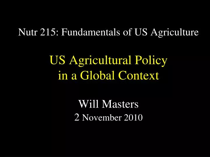
Nutr 215: Fundamentals of US AgricultureUS Agricultural Policy in a Global ContextWill Masters2 November 2010
US Agricultural Policy in a Global Context:What’s ahead today • A lot of data • Three big ideas: • The ‘development paradox’ in government choices, which is paradoxical because of… • The structural transformation in economic activity, and the paradox can be explained by… • The political economy of policy-making. • Ample time for discussion
Where do we see what types of policy? Source: World Bank data, reprinted from UNEP/GRID-Arendal Maps and Graphics Library (http://maps.grida.no/go/graphic/world-bank-country-income-groups).
Poor countries’ governments tax their farmers, while rich countries’ governments subsidize them Average effect of policy on farm product prices, by income level across countries and over time, 1960-2005 Nominal Rate of Assistance to farmers (subsidies or taxes as a proportion of domestic prices) Support for farmers, at the expense of non-farmers (NRA>0 ) Support for non-farmers, at the expense of farmers (NRA<0) ≈ $5,000/yr GDP per person (log scale) Note: Data shown are regression lines and 95% confidence intervals through annual national-average NRAs for over 68 countries, covering more than 90% of world agriculture in each year from 1960 through 2005. Source: W.A. Masters and A. Garcia, “Agricultural Price Distortion and Stabilization: Stylized Facts and Hypothesis Tests,” in K. Anderson, ed., Political Economy of Distortions to Agricultural Incentives. Washington, DC: The World Bank, 2010.
The development paradox also occurs within countries Average Nominal Rate of Protection for Agricultural Production in East Asia, 1955-2002 Source: K. Anderson (2006), “Reducing Distortions to Agricultural Incentives: Progress, Pitfalls and Prospects.” <www.worldbank.org/agdistortions>
As people get richer, what happens to agriculture’s share of employment and earnings? Source: Reprinted from World Bank, World Development Report 2008. Washington, DC: The World Bank (www.worldbank.org/wdr2008)
Some of the transition from farming to nonfarm work is within agriculture, to specialized ‘agribusiness’ Source: Reprinted from World Bank, World Development Report 2008. Washington, DC: The World Bank (www.worldbank.org/wdr2008)
Percent of workforce by sector in the United States, 1800-2005 As the U.S. became richer, what’s happened to agriculture’s share of employment and earnings? today, about 80% of jobs are in services in 1800, employment was 90% farming in 1930s-70s, industry reached about 40% agricultural employment has stabilized Source: U.S. Economic Report of the President 2007 (www.gpoaccess.gov/eop)
Percent of GDP by sector in Australia, 1901-2000 This “structural transformation” out of agriculture, into industry and then services, occurs everywhere Source: Government of Australia (2001), Economic Roundup – Centenary Edition, Department of the Treasury, Canberra.
As agriculture’s share of the economy declines, do farmers’ incomes also decline? Agricultural Employment as a Share of Civilian Employment and Real Farm Output as a Share of Real GDP Until the 1930s, employment and output fell together and then both stopped falling …then employment fell much faster than output SOURCE: U.S. Department of Commerce and the Federal Reserve Bank of St. Louis. Reprinted from K.L. Kliesen and W. Poole, 2000. "Agriculture Outcomes and Monetary Policy Actions: Kissin' Cousins?" Federal Reserve Bank of Sf. Louis Review 82 (3): 1-12.
Percent of non-farm income Thousands of 1992 dollars per farm In the U.S., farm incomes fell and then rose, both absolutely and relative to nonfarm earnings then caught up Farm income fell… Source: BL Gardner, 2000. “Economic Growth and Low Incomes in Agriculture.” AJAE 82(5): 1059-1074.
The same pattern holds across countries: as national income rises, farm incomes fall then rise The farm-nonfarm earnings gap in 86 countries, 1965-2000 The gap worsens as incomes rise, then farmers catch up Source: C.PeterTimmer, A World without Agriculture: The Structural Transformation in Historical Perspective. AEI Press, 2009 (www.aei.org/book/100002).
The story so far… • Poor countries tax farmers and help non-farmers, while rich countries do the reverse • This is paradoxical, because in poor countries • Most people are farmers (so we’d expect them to be influential) • Farmers are relatively poor (so we’d expect them to be helped) • The underlying shift is “structural transformation” • Farming’s share of employment & earnings decline • Farmers’ incomes fall and then rise • What can explain these changes?
What can explain the structural transformationfrom agriculture to industry and then services? • Consumers’ income growth? • Engel’s law and Bennett’s law: as income grows, • demand for food rises less than for other things • demand for staple foods rises less than for higher-value foods • Farmers’ new technology? • Cochrane’s Treadmill: new farm technologies • increase output, lower prices and “push” farmers out • Both of these can explain transformation only when there’s no trade, or for the world as a whole
When there’s international trade, structural transformation can be explained by: • Consumers’ income growth & new farm technology (can explain transformation only for the world as a whole) • Non-farm technology? • The bright lights of the big city • offer an easier life and higher incomes, so “pull” farmers out • Limited farmland? • When individual farmers succeed, they must either • buy/rent land from neighbors, or invest in non-farm activity • People are continually choosing how much land to farm • income from farming is: acres/worker X income/acre farmers leave ag. ASAP, until incomes equalize
The number of farmers rises at first, then falls until farm income matches nonfarm earnings The textbook picture of structural transformation within agriculture: farm numbers stabilized by off-farm income and rising profits per acre; latest census shows slight rise in no. of farms Figure 5-3. Number and average size of farms in the United States, 1900-2002.
Percent of non-farm income Thou. of 1992 dollars per farm The change in acreage per farm is closely linked to farm income
Why does the number of farmers risebefore it falls? • This is very simple, but very surprising: • Is it because of total population growth? • Yes, but usually urban population growth is even faster. • But rural growth also depends on the initial urbanization level: • If we divide the total workforce into farmers and nonfarmers: • Lf = Lt– Ln (Li=no. of workers in sector i) • And solve for the growth rate of the number of farmers: • %Lf = (%Lt – [%Ln•Sn]) / (Sf) (Si=share of workers in i) • We see: Urbanization level (note: Sf +Sf=100%) Rural pop. growth rate Total pop. growth rate Urban pop. growth rate
Why does the number of farmers risebefore it falls? • Applying the formula we just derived: • %Lf = (%Lt – [%Ln•Sn]) / (Sf) (Si=share of workers in i) • We see that even if non-farm employment grows very fast, • the number of farmers may still rise quickly: This rise continues until cities become large and fast-growing enough to absorb all of the total population growth… …then this decline continues until farm & nonfarm incomes equalize
The rise and eventual fall in number of farmers occurs faster/earlier in more prosperous regions Source: Reprinted from W.A. Masters, 2005. “Paying for Prosperity: How and Why to Invest in Agricultural R&D in Africa.” Journal of International Affairs 58(2): 35-64.
The structural transformation is closely linked to differences and changes in government policy Average NRAs for all products by year, with 95% confidence bands Source: Kym Anderson et al., 2009. Distortions to Agricultural Incentives database (www.worldbank.org/agdistortions). Notes: Each line shows data from all available countries in each year from 1961 to 2005 (total n=2520), smoothed with confidence intervals using Stata’slpolyci. Income per capita is expressed in US$ at 2000 PPP prices.
How do we even know what governments doto influence food prices and farm income? • We can imagine two possible approaches: • Add up influence of observed tariffs, subsidies and other transfers • This is the OECD’s “Producer Subsidy Equivalent” approach • Works well for industrialized countries that are subsidizing agriculture • Infer influence from observed market prices • This is the World Bank’s tariff-equivalent “distortions” approach • Needed to compare large numbers of developing and developed countries • Both approaches lead to the same answer: • Policy effects are differences between domestic and foreign prices • Policy effects = domestic prices – foreign prices ± cost of transport etc. • Domestic prices may be raised or lowered by policy • Foreign prices are each product’s opportunity cost in trade
- P P dom free º NRA P free Notation for the tariff-equivalence approachto policy measurement, used by World Bankfor Distortions to Agricultural Incentives • Tariff-equivalent ‘Nominal Rate of Assistance’ in domestic prices relative to free trade: • Occasionally estimated directly from observed policy: • More often imputed by price comparison:
Procedures and results fromDistortions to Agricultural Incentives • A 3-year project: • 100+ researchers and case studies for 68 countries, 77 commodities over 40+ years; in total have over 25,000 policy measurements. • Project results published in six books • Four volumes of country narratives • Africa, Asia, LAC and European Transition • Two global volumes • Regional syntheses and simulations • Political economy explanations for policy choices • Some of today’s results are from W.A. Masters and A.F. Garcia (2010), “Agricultural Price Distortion and Stabilization: Stylized Facts and Hypothesis Tests,” in K. Anderson, ed., Political Economy of Distortions to Agricultural Incentives. Washington, DC: World Bank. • All available as e-books at www.worldbank.org/agdistortions
Commodities covered by Distortions to Agricultural Incentives Note: Totals above are for the top 30 global commodities; An additional 47 other products also appear in the dataset.
The results: Distortions have grown and shrank Constant 2000 US$ (billions) Source: Anderson, K. (forthcoming), Distortions to Agricultural Incentives: A Global Perspective, 1955 to 2007, London: Palgrave Macmillan and Washington DC: World Bank.
Policy reforms have reduced both anti-farm and anti-trade biases Developing countries Importables Total 0 Exportables Percent This gap is anti-trade bias This level is anti-farm bias High-income countries plus Europe’s transition economies High-income countries’ biases have also shrunk Importables Percent Total Exportables 0 Source: Anderson, K. (forthcoming), Distortions to Agricultural Incentives: A Global Perspective, 1955 to 2007, London: Palgrave Macmillan and Washington DC: World Bank.
On average, Africa has had very large and sustained reforms since the 1990s Importable products Smaller anti-trade bias since 1990s All farm products Exportable products Smaller anti-farm bias Source: K.Anderson and W. Masters (eds), Distortions to Agricultural Incentives in Africa. Washington, DC: The World Bank, 2009.
Asia has large pro-farm shift; ending net export taxes in 1990s, net support to ag. since 1980s Importable products All farm products No more net export taxation since 1990s Exportable products No more anti-farm bias since 1980s Source: K.Anderson and W. Martin (eds), Distortions to Agricultural Incentives in Asia. Washington, DC: The World Bank, 2009.
Latin America has had similar trends at a slower pace,supporting ag. since 1990s Importable products All farm products Exportable products Source: K.Andersonand A. Valdes (eds), Distortions to Agricultural Incentives in Latin America. Washington, DC: The World Bank, 2009.
Reform paths vary within regionsExamples in Africa Countries’ total NRA for all tradable farm products, 1955-2004
Reform paths vary within regionsExamples in Asia Countries’ total NRA for all tradable farm products, 1955-2004
Reform paths vary within regionsExamples in Latin America Countries’ total NRA for all tradable farm products, 1955-2004
Reform paths vary within regionsExamples among High-Income Countries Countries’ total NRA for all tradable farm products, 1955-2004
To explain and predict policy change, we’ll need to merge regions and test hypotheses A key variable will be per-capita income National average NRAs by real income per capita, with 95% confidence bands Anti-farm bias ends at about $5,000/yr Anti-trade bias ends above $12,000/yr (≈$400/yr) (≈$3,000/yr) (≈$22,000/yr) Source: Author’s calculations, from data available at www.worldbank.org/agdistortions. Each line shows data from 66 countries in each year from 1961 to 2005 (n=2520), smoothed with confidence intervals using Stata’s lpolyci at bandwidth 1 and degree 4. Income per capita is expressed in US$ at 2000 PPP prices.
To explain and predict policy, we’ll need to think carefully about who benefits
Farm policy is not a pretty sight! Note this cartoon is from the U.S. in 2002; similar farm policies are supported by all political parties.
Modern political economy:Two main theories • ‘Positive’ or ‘neoclassical’ political economy focuses on: • government as a marketplace for competing interests, where • observed policies reveal the balance of power, and • power results from people (or firms) deciding to invest in politics • Why would some invest more than others in politics? • If the answer were just income and wealth, we’d see free trade! • To explain what we actually see, two of the main theories are: • Size of potential gains from politics (per person or per firm) • Larger impact = more incentive to invest • Small impacts = ‘rational ignorance’? (Downs 1954) • Size of interest group (number of people or firms) • Larger group = more ‘free-ridership’ (Olson 1965) • Smaller group = easier cooperation, but offset by fewer votes?
Modern political economy:Size of gains and the rational ignorance of losers • The basic idea of “rational ignorance” is that • learning about and participating in political action is costly, • so people won’t, unless it’s worthwhile to do so • Some implications of this model are that: • only those with relatively large stakes will participate in politics; • if people have similar and large stakes, they can lobby together; • the costs of participation can have a decisive influence; • if political information is easier to get, and • if political participation is easier to do, • then outcomes will be more economically efficient • …but participants in politics may deliberately choose confusing and ambiguous policies, to raise the costs of participation!
Modern political economy:Size of interest groups and free ridership • The basic idea of the “interest-group” approach is that • policy choices are inherently collective actions, • so obtaining desired policies requires limiting free-ridership • Some implications of the interest-group approach are that people will invest more in politics if they: • are few in number (so each is less likely to free-ride) • are fixed in number (so new entrants won’t free-ride)
Modern political economy:Five other theories • Rent seeking • Mainly due to Anne Krueger (1974) on Turkish trade policy • Checks and balances can offset interest groups • Time consistency • Due to Kydland and Prescott (1977) on inflation and central banks • Government can do only what it can credibly commit to keep doing • Loss aversion • Due to Kahnemann and Tversky (1979) in psychology • People hate losses more than they love gains • The resource curse • Many authors, mainly from experience with minerals and oil • Governments exploit what’s abundant • Anti-trade bias and revenue motives • Many authors: governments tax what they can • Of course there are also plenty of other, less influential theories…
Results: The stylized facts in OLS regressions Table 1. Stylized facts of observed NRAs in agriculture The development paradox The resource curse Some regional differences Anti-trade bias
Results:Specific hypotheses at the country level Table 2. Hypothesis tests at the country level Revenue Motives Rent dissipation Rational ignorance Number of people Rentseeking
Results:Specific hypotheses at the product level Table 3. Hypothesis tests at the product level Time consistency Loss aversion
More results: Since 1995, policies have moved closer to free-trade prices National average NRAs by income level, before and after the Uruguay Round agreement Flatter curves, closer to zero