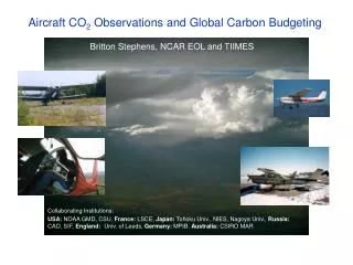
Light Aircraft CO 2 Observations and the Global Carbon Cycle

1. Light Aircraft CO2 Observations and the Global Carbon Cycle Britton Stephens, NCAR EOL and TIIMES Collaborating Institutions: USA: NOAA GMD, CSU, France: LSCE, Japan: Tohoku Univ., NIES, Nagoya Univ., Russia: CAO, SIF, England: Univ. of Leeds, Germany: MPIB, Australia: CSIRO MAR

2. Expected from fossil fuel emissions Motivation: Atmospheric CO2 increase Climate change

3. Global and hemispheric constraints on the carbon cycle Annual-mean CO2 exchange (PgCyr-1) from atmospheric O2 TransCom1 fossil-fuel gradients Surface Observations

4. [courtesy of Scott Denning]

5. Seasonal vertical mixing [courtesy of Scott Denning]

6. Transcom3 neutral biosphere flux response ppm Latitude

7. TransCom3 model results based on surface data imply a large transfer of carbon from tropical to northern land regions. Level 1 (annual mean) Level 2 (seasonal) Gurney et al, Nature, 2002 Gurney et al, GBC, 2004

8. Bottom-up estimates have failed to find large uptake in northern ecosystems and large net sources in the tropics

9. Transcom 3 Level 2 annual-mean model fluxes fluxes in PgCyr-1 = GtCyr-1 = “billions of tons of C per year” @ $3 - $30 / ton, 3 PgCyr-1 ~ $10 - $100 billion / year

10. Impact on predicted fluxes TransCom3 predicted seasonal effects explain most of the variability in estimated fluxes. Response to neutral biosphere flux

11. Transcom3 neutral biosphere flux response pressure N S N S N S N S ppm

12. Map of airborne flask sampling locations Northern Hemisphere sites include Briggsdale, Colorado, USA (CAR); Estevan Point, British Columbia, Canada (ESP); Molokai Island, Hawaii, USA (HAA); Harvard Forest, Massachusetts, USA (HFM); Park Falls, Wisconsin, USA (LEF); Poker Flat, Alaska, USA (PFA); Orleans, France (ORL); Sendai/Fukuoka, Japan (SEN); Surgut, Russia (SUR); and Zotino, Russia (ZOT). Southern Hemisphere sites include Rarotonga, Cook Islands (RTA) and Bass Strait/Cape Grim, Australia (AIA).

13. Airborne flask sampling data

14. 20 -15 10 -10 10 Altitude-time CO2 contour plots for all sampling locations -10 0 -5

15. Northern Hemisphere average CO2 contour plot from observations

16. Model-predicted NH Average CO2 Contour Plots Observed NH Average CO2 Contour Plot

17. Vertical CO2 profiles for different seasonal intervals

18. Observed and predicted NH average profiles

19. Estimated fluxes versus predicted 1 km – 4 km gradients • 3 models that most closely reproduce the observed annual-mean vertical CO2 gradients (4, 5, and C): • northern land uptake = -1.5 ± 0.6 PgCyr-1 • tropical land emission = +0.1 ± 0.8 PgCyr-1 • All model average: • northern land uptake = -2.4 ± 1.1 PgCyr-1 • tropical land emission = +1.8 ± 1.7 PgCyr-1 Observed value

20. Observational and modeling biases evaluated: • Interlaboratory calibration offsets and measurement errors • Diurnal biases • Interannual variations and long-term trends • Flight-day weather bias • Spatial and Temporal Representativeness All were found to be small or in the wrong direction to explain the observed annual-mean discrepancies

21. Estimated fluxes versus predicted 1 km – 4 km gradientsfor different seasonal intervals Observed values

22. Should annual-mean or seasonal gradients be used to evaluate models? • Annual-mean fluxes are of most interest because they are relevant to annual ecosystem budgeting, to policy makers, and to projections of future greenhouse gas levels • No model does well at all times of year. Models that do well in summer do poorly in other seasons. • Errors in seasonal timing of fluxes make selection of seasonal criteria problematic • Seasonal effects are inherently cumulative, such that a model with large seasonal errors that offset will do better in annual-mean that one with small seasonal errors that compound.

23. Conclusions: • Models with large tropical sources and large northern uptake are inconsistent with observed annual-mean vertical gradients. • A global budget with less tropical  north carbon transfer is also more consistent with bottom-up estimates and does not conflict with independent global 13C and O2 constraints. • Simply adding airborne data into the inversions will not necessarily lead to more accurate flux estimates • Models’ seasonal vertical mixing must be improved to produce flux estimates with high confidence • There is value in leaving some data out of the inversions to look for systematic biases

24. What is the role for heavier and lighter aircraft? • Continuous instrumentation • Multiple species • Long-range operations • Boundary-layer intensives • Low-altitude flux legs

25. a) b) CO2 [ppm] CO [ppb] c) d) CO2 [ppm] CO [ppb] COBRA-NA 2000 CO2 CO North South

26. Airborne Carbon in the Mountains Experiment (ACME-04) All flights: Transport Predictions and CO2 Profiles for July 29, 2004 First-Order Regional CO2 Flux Estimates

27. S S S N N N HIAPER Pole-to-Pole Observations of Atmospheric Tracers HIPPO (PIs: Harvard, NCAR, Scripps, and NOAA): A global and seasonal survey of CO2, O2, CH4, CO, N2O, H2, SF6, COS, CFCs, HCFCs, O3, H2O, and hydrocarbons Fossil fuel CO2 gradients over the Pacific UCI UCIs pressure N S N S JMA MATCH.CCM3 pressure N S N S ppm

28. Aircraft Data Providers: Pieter P. Tans, Colm Sweeney, Philippe Ciais, Michel Ramonet, Takakiyo Nakazawa, Shuji Aoki, Toshinobu Machida, Gen Inoue, Nikolay Vinnichenko, Jon Lloyd, Armin Jordan, Martin Heimann, Olga Shibistova, Ray L. Langenfelds, L. Paul Steele, Roger J. Francey TransCom3 Modelers: Kevin Robert Gurney, Rachel M. Law, Scott Denning, Peter J. Rayner, David Baker, Philippe Bousquet, Lori Bruhwiler, Yu-Han Chen, Philippe Ciais, Inez Y. Fung, Martin Heimann, Jasmin John, Takashi Maki, Shamil Maksyutov, Philippe Peylin, Michael Prather, Bernard C. Pak, Shoichi Taguchi