Tsuyoshi Yamamoto
510 likes | 687 Vues
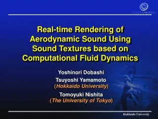
Yoshinori Dobashi. Tsuyoshi Yamamoto. ( Hokkaido University ). Tomoyuki Nishita. ( The University of Tokyo ). Real-time Rendering of Aerodynamic Sound Using Sound Textures based on Computational Fluid Dynamics. Hokkaido University. http://nis-ei.eng.hokudai.ac.jp/~doba.

Tsuyoshi Yamamoto
E N D
Presentation Transcript
Yoshinori Dobashi Tsuyoshi Yamamoto (Hokkaido University) Tomoyuki Nishita (The University of Tokyo) Real-time Rendering of Aerodynamic Sound Using Sound Textures based on Computational Fluid Dynamics
Hokkaido University http://nis-ei.eng.hokudai.ac.jp/~doba Examples of aerodynamic sound • Sound of wind • Sound generated by swinging objects quickly
Overview • Introduction • Related Work • Principle and Prediction of Aerodynamic Sound • Basic Idea of Our Method • Computation of Sound Texture • Real-time Sound Rendering • Examples • Conclusions
Overview • Introduction • Related Work • Principle and Prediction of Aerodynamic Sound • Basic Idea of Our Method • Computation of Sound Texture • Real-time Sound Rendering • Examples • Conclusions
Introduction • Simulation of virtual environments • Sound: important element • voice, contact sound, etc. • Improving reality of virtual environments • Use of recorded sound • need to find suitable sound • quality depends on environment
Introduction • Physically-based sound synthesis • compute waves based on physical simulation • generate sound automatically according to object motion • Limited to sound due to solid objects • Sound due to fluid • wind(aerodynamic sound), water, explosion ...
Goal and Feature • Real-time rendering of aerodynamic sound • source is not oscillation of solid objects • creating sound textures for aerodynamic sound • rendering sound in real-time according to object motion
Goal and Feature • Sound by swinging sword and club • Real-time sound rendering • Sound synthesis depending on shapes and motion of objects
Overview • Introduction • Related Work • Principle and Prediction of Aerodynamic Sound • Basic Idea of Our Method • Computation of Sound Texture • Real-time Sound Rendering • Examples • Conclusions
Related Work in CG [Takala92] [Funkhouser99] [Tsingos01] • Propagation of sound • simulate reflection/absorption due to objects to compute sound taking into account geometric relation between source and receiver [Hahn95][O’Brien01][O’Brien02][van den doel01] • Synthesis of sound waves • compute sound waves by numerical analysis of subtle oscillation of objects • No methods for aerodynamic sound
Related Work in CFD • Prediction of aerodynamic sound [Lele97] • to reduce noise due to high-speed transportation facilities, etc. • complex numerical fluid simulation • not appropriate for real-time applications • Our method… • Makes use of methods developed in CFD • Realizes real-time sound synthesis
Overview • Introduction • Related Work • Principle and Prediction of Aerodynamic Sound • Basic Idea of Our Method • Computation of Sound Texture • Real-time Sound Rendering • Examples • Conclusions
cylinder flow Principle and Prediction • Source of aerodynamic sound vortices • vortices in air • subtle fluctuations of air pressure due to vortices • Prediction method • Lighthill’s basic theory in 1952 [Ligh52] • numerical simulation of compressibleNavier-Stokes equations → computationally expensive • Curle’s model
pa sound source field sound object r vortex receiver q flow Incompressible fluid analysis center position o Curle’s Model • Prediction by behavior of air near object
Curle’s Model • Prediction by behavior of air near object
amp. time flow sound source field Curle’s Model • Prediction by behavior of air near object sound source function (SSF) normal pressure g(t) (x component)
sound pressure pa sound source field r receiver q g(t) flow center position o Curle’s Model • Prediction by behavior of air near object sound source function (SSF)
constraint:Size of object must be sufficiently small relative to wavelength of sound Curle’s Model • Prediction by behavior of air near object sound source function (SSF)
Overview • Introduction • Related Work • Principle and Prediction of Aerodynamic Sound • Basic Idea of Our Method • Computation of Sound Texture • Real-time Sound Rendering • Examples • Conclusions
region 1 receiver q virtual sound source + region 2 region n Basic Idea • Use of Curle‘s model • not applicable to large object • subdivide object into small regions • equivalent to assuming independent virtual point sound sources
Basic Idea • Computing sound texture (preprocess) • Rendering aerodynamic sound (real-time)
s:time in texture domain t:time in reality l SSF table speed v uniform flow direction u speed v time s sound source pos. l fluid analysis sound texture: w(l, s, u, v) Basic Idea • Computing sound texture (preprocess) • fluid analysis → table of sound source func. • Rendering aerodynamic sound (real-time)
l flow direction u speed v fluid analysis sound texture: w(l, s, u, v) Basic Idea • Computing sound texture (preprocess) • fluid analysis → table of sound source func. • Rendering aerodynamic sound (real-time)
l l move c1 v1 c2 v2 cn vn (sound texture) Basic Idea • Computing sound texture (preprocess) • fluid analysis → table of sound source func. • Rendering aerodynamic sound (real-time) • dir./speed →values of SSF →sound texture SSF values (g1, g2, …, gn) receiver pos. q
sound wave Basic Idea • Computing sound texture (preprocess) • fluid analysis → table of sound source func. • Rendering aerodynamic sound (real-time) • dir./speed →values of SSF →sound texture → sound pressure →Curle’s model SSF values (g1, g2, …, gn) Curle‘s model receiver pos. q
sound wave Basic Idea • Computing sound texture (preprocess) • fluid analysis → table of sound source func. • Rendering aerodynamic sound (real-time) • dir./speed →values of SSF →sound texture → sound pressure →Curle’s model SSF values (g1, g2, …, gn) Curle‘s model receiver pos. q
Overview • Introduction • Related Work • Principle and Prediction of Aerodynamic Sound • Basic Idea of Our Method • Computation of Sound Texture • Real-time Sound Rendering • Examples • Conclusions
fluid analysis speed v time s flow dir. u speed v sound source pos.l sound texture Computation of Sound Texture • Fluid analyses for many directions and speeds • long computation time
fluid analysis speed v time s v0 flow dir. u speed v sound source pos.l sound texture Computation of Sound Texture • Properties of aerodynamic sound • frequency ∝ flow speed v • amplitude ∝ (flow speed v )6 • Need only sound texture at base speed v0 • Reduce computation time and memory requirement drastically
speed v time cross section v0 y sound source pos. flow x 2D analysis Choosing 2D or 3D Fluid Analysis Stick-like object
Stick-like object cross section y flow x 2D analysis Choosing 2D or 3D Fluid Analysis speed v time v0 sound source pos. 1D sound tex.
time point sound source flow 1 direction 1 2 2 3 3 speed v time point sound source v0 sound source pos. 3D analysis Choosing 2D or 3D Fluid Analysis Stick-like object 1D sound tex. 2D sound tex. 2D analysis Others 2D sound tex.
Stick-like object time 3 3 2 2 point sound source 1 1 1 direction 1D sound tex. 2D sound tex. 2D analysis 1 2 2 3 3 Others Choosing 2D or 3D Fluid Analysis 2D sound tex. 3D analysis
Stick-like object time 3 2 point sound source 1 1 direction 1D sound tex. 2D sound tex. 2D analysis 1 2 2 3 3 time direction Others sound source pos. Choosing 2D or 3D Fluid Analysis 3D sound tex. 2D sound tex. 3D analysis
Overview • Introduction • Related Work • Principle and Prediction of Aerodynamic Sound • Basic Idea of Our Method • Computation of Sound Texture • Real-time Sound Rendering • Examples • Conclusions
Real-time Sound Rendering • Procedure - repeat for each time step Dt
move c1 v1 c2 v2 cn vn Real-time Sound Rendering • Procedure - repeat for each time step Dt 1. compute direction ci and speed vi
soundtexture direction (c1, c2, …, cn) speed (v1, v2, …, vn) w(l, s, u, v0) values of SSF (g1, g2, …, gn) Real-time Sound Rendering • Procedure - repeat for each time step Dt 1. compute direction ci and speed vi 2. compute SSF gi
r1 r2 rn Real-time Sound Rendering • Procedure - repeat for each time step Dt 1. compute direction ci and speed vi 2. compute SSF gi 3. compute distance ri to receiver
+ Real-time Sound Rendering • Procedure - repeat for each time step Dt 1. compute direction ci and speed vi 2. compute SSF gi 3. compute distance ri to receiver 4. compute sound pressure pv Curle‘s model
soundtexture direction (c1, c2, …, cn) speed (v1, v2, …, vn) w(l, s, u, v0) (texture for base speed) values of SSF (g1, g2, …, gn) Real-time Sound Rendering • Procedure - repeat for each time step Dt 1. compute direction ci and speed vi 2. compute SSF gi 3. compute distance ri to receiver 4. compute sound pressure pv
vi actual speed Dt t s w sound texture (base speed v0) Computation of SSF • Property • freq. ∝ speed v • amp. ∝ (speed v )6
Property • freq. ∝ speed v • amp. ∝ (speed v )6 different interval Computation of SSF vi actual speed vi(k) Dt k t s w sound texture (base speed v0)
Property • freq. ∝ speed v • amp. ∝ (speed v )6 Computation of SSF vi actual speed vi(k) Dt k t x(vi(k)/v0)6 s vi(k)/v0xDt w sound texture (base speed v0)
Property • freq. ∝ speed v • amp. ∝ (speed v )6 = D + ì s ( v ( t ) / v t ) s ï - k l k 0 k 1 í 6 = ï g ( t ) ( v ( t ) / v ) w ( l , s , c , v ) î l k l k 0 k l 0 w overlap Computation of SSF vi actual speed Dt • Recurrence relation t s w • Periodical use • blending for smooth transition sound texture (base speed v0)
Overview • Introduction • Related Work • Principle and Prediction of Aerodynamic Sound • Basic Idea of Our Method • Computation of Sound Texture • Real-time Sound Rendering • Examples • Conclusions
Fluid Simulation Demo • Sound texture for square prism for one direction of flow • length 50cm, side length 2.0cm • base speed 10 m/s • 2D analysis • finite difference
Rotating sphere • wire has no effect on sound • Doppler effect • Cylinder thrown at receiver • rotating as it approaching • Doppler effect • Sound by wind • wind through fence • draft through gap between windows Real-time Sound Rendering Demo
Application • Character animation • Bear swinging a huge club • Warrior swinging two different swords (image by TAITO)
Conclusions • Sound synthesis of fluid • Real-time rendering of aerodynamic sound • sound texture based on CFD • synthesis of sound waves using Curle‘s model • real-time • New element to improve realistic simulation of virtual environments