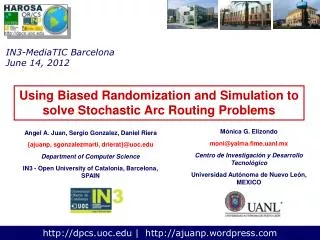
Using Biased Randomization and Simulation to solve Stochastic Arc Routing Problems
IN3-MediaTIC Barcelona June 14, 2012. Using Biased Randomization and Simulation to solve Stochastic Arc Routing Problems. Mónica G. Elizondo moni@yalma.fime.uanl.mx Centro de Investigación y Desarrollo Tecnológico Universidad Autónoma de Nuevo León, MEXICO.

Using Biased Randomization and Simulation to solve Stochastic Arc Routing Problems
E N D
Presentation Transcript
IN3-MediaTIC Barcelona June 14, 2012 Using Biased Randomization and Simulation to solve Stochastic Arc Routing Problems Mónica G. Elizondo moni@yalma.fime.uanl.mx Centro de Investigación y Desarrollo Tecnológico Universidad Autónoma de Nuevo León, MEXICO Angel A. Juan, Sergio Gonzalez, Daniel Riera {ajuanp, sgonzalezmarti, drierat}@uoc.edu Department of Computer Science IN3 - Open University of Catalonia, Barcelona, SPAIN http://dpcs.uoc.edu | http://ajuanp.wordpress.com
4 3 5 2 0 6 1 7 1. The Capacitated ARP (deterministic) Edges withdemands Nodes • The Capacitated Arc Routing Problem (CARP) is a well-known NP-hard problem Golden et al. (1981): • The set of edges constitute an undirected, non-complete graph or network. • A set of edges’ demands must be supplied by a fleet of (homogeneous) vehicles. • Resources are available from a depot. • Moving a vehicle from one node i to another j has associated (symmetric) costsc(i, j) > 0. • An edge might be traversed several times by different vehicles, but it is served by just one vehicle. • Additional constraints must be considered: maximum load capacity per vehicle, service times, etc. Depot (resources) • Goal: to obtain an ‘optimal’ solution, i.e. a set of routes satisfying all constraints with minimum costs
4 3 5 2 0 6 1 7 2. Variants of the CARP • Different ARP variants have been proposed: • Directed CARP (DCARP): A version of the CARP where the Arcs can be traversed in a single direction (Maniezzo & Roffilli, 2008). • Mixed CARP (MCARP): A version of the CARP with mixed graphs (Belenguer, Benavent, Lacomme, & Prins, 2006). • Min-Max k-CPP: CARP-like problem excluding capacity constraints on vehicles (Ulusoy, 1985). • Periodic CARP (PCARP): CARP extended to the planning of P days (Lacomme, Prins, Ramdane-Chérif, 2002). • CARP with Stochastic demands (ARPSD): CARP where the demand to be served is not known beforehand (Fleury, Lacomme, & Prins, 2005). • Etcetera.
4 3 5 2 0 6 1 7 3. Practical Applications • Some ARP practical applications are: • Refuse collection(Almeida & Mourão, 2000). • Snow removal (Eglese, 1994). • Inspection of distributed systems (Lee, 1989). • Routing of electric meter readers (Stern & Dror, 1979). • School bus routing (Ferland & Gudnette, 1990).
4. Solving Approaches (1/2) • Exact Methods (optimal solutions for small-scale problems): • Branch and Bound techniques (Kiuchi, Hirabayashi, Saruwatari, & Shinano, 1995). • Tour construction algorithms (Hirabayashi, Nishida, & Saruwatari, 1992). • Subtour elimination algorithms (Saruwatari, Hirabayashi, & Nishida, 1992). • ILP formulations (Belenguer & Benavent, 1992). • Heuristics (fast, ‘good’ solutions) : • Path Scanning algorithm, Augment-Merge algorithm, Construct-Strike algorithm (Golden, DeArmon, & Baker, 1983). • Node duplication heuristic (Wøhlk, 2005). • The Cycle Assignment algorithm (Benavent, Campos, Corberan, & Mota, 1990). • Parallel insert algorithm (Chapleau, Ferland, Lapalme, & Rousseau,1984).
4. Solving Approaches (2/2) • Meta-heuristics (pseudo-optimal solutions): • Tabu Search algorithms (Hertz, Laporte, & Mittaz, 2000; Greistorfer, 2003). • Simulated Annealing (Eglese, 1994). • Genetic Algorithms (Lacomme, Prins, & Ramdane-Chérif, 2001). • Ant Colony Optimization (Lacomme, Prins, & Tanguy, 2004). • Memetic Algorithms (Lacomme, Prins, & Ramdane-Chérif, 2004).
5. Our SHARP procedure for the CARP • Based on the savings heuristic for the CVRP (Clarke & Wright, 1964). • Designed to provide a ‘good’ starting point for CARP metaheuristics. • SHARP main steps: • Use the Floyd-Warshall algorithm to compute the shortest paths for all pairs of nodes in the network. This allows to treat the graph as if it was a complete one. • Compute the savings associated with demanding edges (real or virtual) connecting any two nodes and create a sorted savings list. • Create a dummy (initial) solution by assigning a route to each demanding arc. • Iterate over the list of savings and look at each node in the selected arc to see which routes (if any) have that node as an exterior node, attempting to merge these routes if possible. • Reconstruct the final solution by computing the shortest path between the edges in the route. Gonzalez, S.; Juan, A.; Riera, D.; Castella, Q.; Muñoz, R.; Perez, A. (in press): “Development and Assessment of the SHARP and RandSHARP algorithms for the Arc Routing Problem”. AI Communications.
6. RandSHARP: a Multi-Start approach • SHARP the first edge (the one with the most savings) is the one selected. • RandSHARP introduces randomness in this process by using a quasi-geometric statistical distribution edges with more savings will be more likely to be selected at each step, but all edges in the list are potentially eligible. • Notice: Each time RandSHARP is run, a random feasible solution is obtained. By construction, chances are that this solution outperforms the SHARP one hundreds of ‘good’ solutions can be obtained after some seconds/minutes. Good results with 0.10 < α < 0.20 Juan, A.; Faulin, J.; Jorba, J.; Riera, D.; Masip; D.; Barrios, B. (2011): “On the Use of Monte Carlo Simulation, Cache and Splitting Techniques to Improve the Clarke and Wright Savings Heuristics”. Journal of the Operational Research Society, Vol. 62, pp. 1085-1097.
7. Computational Experiments RandSHARP >> RandPSH >> SHARP >> PSH
8. The ARP with Stochastic Demands • Important observations: • The random behavior of edges’ demands could cause an expected feasible solution to become an infeasible one if the final demand of any route exceeds the actual vehicle capacity route failure • Corrective actionsmust be introduced to deal with route failures. These actions (e.g. a vehicle reload at the depot) will increase the total expected costs Route failures corrective/preventive policies increase in variable costs E[Total Costs] = Total Fixed Costs + E[Variable Costs] • Goal: to construct reliable solutions with a given probability of suffering route failures • How?:to construct routes in which the associated expected demand will be somewhat lower than the vehicle capacity, i.e., use a safety stock (extensively used in inventory-related problems) • But… be careful: a trade-off exists between routes’ reliability and (fixed) costs minimization Safety stocks in routing
9. Sequential approach for the ARPSD (1/2) Given a ARPSD instance n edges, random demands Di and VMC Set a value for k (0 < k <= 1), the % of the VMC that will be used during the design stage, and set VMC* = k*VMC (i.e.: safety stock = (1 – k)*VMC) Define the CARP(k) with VMC* and di* = E[Di] First solve CARP, then apply MCS • Solve the CARP(k) by using the RandSHARP algorithm. Notice that: • The solution for CARP(k) is also a feasible solution for the ARPSD as far as no route failures occur • The costs of CARP(k) are the fixed costs for the ARPSD • Chances are that some route failures occur (more as k gets closer to 1), so expected variable costs must be also considered ( E[TC] = TFC + E[VC] )
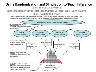
9. Sequential approach for the ARPSD (2/2) • From the CARP(k) solution, estimate the E[VC] due to route failures by using MCS: • Random demands are generated and whenever a route failure occurs, a corrective policy ( costs) is applied • From the CARP(k) solution, obtain an estimate for the reliability of each route, Rj(1 <= j <= m) by using MCS: • Route reliability = probability that the j-th route will not suffer a failure, i.e.: that the j-th vehicle will not run out of load First solve CVRP, then apply MCS Obtain an estimate for the solution reliability. If demands are independent, solution reliability is the product of the Rj Repeat from Step 1 with a new value of k, i.e.: explore different k-based scenarios Provide a sorted list with the best ARPSD solutions found as well as their properties (E[TC], TFC, E[VC], reliability index, etc.)
10. Parallel approach for solving the ARPSD Integrate MCS into the RandSHARP • Parallelization: • Each stock-related scenario can be run in a different processor. • At the end, the ‘best’ scenario (the one with the best found solution) is selected. • For each scenario (stock level): • Consider the associated CARP problem. • Assign the scenario to a new processing unit. • Solve it by using the RandSHARP with MCS. • Save the associated solution.
11. Advantages of our Approach • The idea of solving the VRPSD through solving a related CVRP is not new (Fleury et al. 2005). However, our approach differs from others in: • It contemplates the analysis of different risk scenarios or CARP(k) • It uses a more practical perspective based on the combination of MCS and reliability analysis • It does not require from strong assumptions on the variables that model customers’ demands • Potential benefits: • Wider scope: it is valid for any statistical distribution with a known mean • Efficiency: it reduces the complexity of a VRPSD to a more tractable CVRP • Flexibility: it offers different risk-based scenarios to the decision-maker
Gap between the CARP(k) solution obtained with RandSHAP and the CARP(k) solution obtained by using SHARP 12. Expected results Solution 2 is the one with the lowest E[TC] Notice: the number of necessary routes increases as k decreases (since safety stocks = 1 – k) Notice: as k decreases, TFC increases and E[VC] decreases Gives an estimate of the solution’s feasibility-level (as k decreases, the reliability increases since it is more unlikely to suffer route failures)
13. Computational Results (1/2) • Knowing that in the ARPSD literature there are no commonly used benchmarks, many authors construct their own instances, generated using different statistical distributions. • The previous situation implies that many results are dependent on the statistical assumptions. • Now, we have designed a methodology based on introducing randomness in demands of the well-known CARP instances. • We have modeled random demands, Di, considering E[Di] = di (original demands) and Var[Di] = wE[Di] with w= 0 (deterministic problem), w=0.05 (small variance), w=0.25 (moderate variance)or w=0.75 (large variance). Different designs of demands in means and variances.
13. Computational Results (2/2) • In a ARPSD, a scenario with less route failures might provide lower total expected costs.
14. Conclusions • We have presented the SHARP procedure solving the CARP. This procedure is based on the savings heuristic for the CVRP. • We have introduced the RandSHARP algorithm for the CARP. This algorithm uses biased randomization to improve the SHARP procedure. • We have also proposed an approach for solving the ARPSD. This approach combinesMCSwithparallel computing and theRandSHARPalgorithm. • The basic idea is to consider a vehicle capacity lower than the actual VMC when constructing CARP solutions. This way, this capacity surplusorsafety stockscan be used when necessary to significantly reduce the expected costs due to expensiveroute failures. • Our approach provides the decision-maker with a set of alternative solutions with different properties (number of routes, fixed and expected variable costs, reliability indices, etc.) • It offers flexibility since it does not assume any particular behavior of the customers’ stochastic demands. Therefore, the probabilistic distributions which describe demands can be generic. • The randomized algorithm is easily parallelizable, which allows to generate pseudo-optimal solutions in ‘reasonable’ clock times.
IN3-MediaTIC Barcelona June 14, 2012 Using Biased Randomization and Simulation to solve Stochastic Arc Routing Problems Thanks for your attention! Mónica G. Elizondo moni@yalma.fime.uanl.mx Centro de Investigación y Desarrollo Tecnológico Universidad Autónoma de Nuevo León, MEXICO Angel A. Juan, Sergio Gonzalez, Daniel Riera {ajuanp, sgonzalezmarti, drierat}@uoc.edu Department of Computer Science IN3 - Open University of Catalonia, Barcelona, SPAIN http://dpcs.uoc.edu | http://ajuanp.wordpress.com