3D Spectrography: II - The tracers
390 likes | 627 Vues
3D Spectrography: II - The tracers. Morphology : distribution of each component Dynamics : kinematics via the emission or absorption lines Line strengths : allow to study stellar populations. The different tracers: Gas. 90% H, 10% He Neutral, ionized, molecular. H. He. Dust. Mass.

3D Spectrography: II - The tracers
E N D
Presentation Transcript
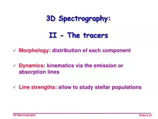
3D Spectrography:II - The tracers • Morphology: distribution of each component • Dynamics: kinematics via the emission or absorption lines • Line strengths: allow to study stellar populations
The different tracers: Gas • 90% H, 10% He • Neutral, ionized, molecular H He Dust Mass Cloud T Density Orion HI HII H2 Dust Msun Msun (K) cm-3
HI Gas • Hyperfine transition line at 21 cm Aligned poles (higher energy) Opposed poles (lower energy) • Rare transition, but very abundant gas
HI Gas • Velocity profiles Sofue et al.
HI Gas • Position-Velocity diagram
HI Gas - Kinematics • NGC 253 – HI Observations Koribalski et al.
Ionized gas: Ha • Spectrum in the visible
Ionized gas: Ha • Comparison HI / Ha
Ionized gas: Ha • Velocity map Khoruzhii et al.
Stars galaxy • Absorption lines template Calcium triplet • Deconvolution: G = S* LOSVD G = S*LOSVD LOSVD : Line Of Sight Velocity Distribution l [ang] LOSVD V [km/s]
Stars • Problems due to population differences (template mismatching) Different populations = Different kinematics • Deconvolution: G = Siai Si* LOSVDi G= Siai Si* LOSVDi
LOSVDs and kinematics • Many different methods for deconvolving: • Direct pixel fitting • Fourier fitting • Cross-correlation techniques • Fourier Quotient Correlation method • Others… • Fittings LOSVD moments: • Gauss-Hermite moments (van der Marel & Franx 93, ApJ 407, 525 Gerhard 93, MNRAS 265, 213)
LOSVDs and kinematics • LOSVDs of NGC 5582 Halliday et al., 2001, MNRAS, 326, 473
LOSVDs and kinematics Halliday et al., 2001, MNRAS, 326, 473
How to determine the age and composition of a galaxy? • Assume1 age and uniform composition. • Assume same laws of physics as in • a globular cluster. • Stellar evolution: artificial HR diagram • Findmatching spectra • Add these spectra composite galaxy spectrum • Repeat previous steps for different ages/metallicities • Determinebest fit
Determining age and metallicity in practice The Lick System of Indices • Determine strengths of absorption features • Correct them for velocity broadening of the galaxy • Compare them with theoretical line strengths
Stellar population models Vazdekis (1999) models at Lick resolution (~9 Å FWHM) based on Jones (1999) library [MgFe52]=(Mgb x Fe5270)^0.5
Age & metallicity for Fornax galaxies Kuntschner 2000, MNRAS, 315, 184
Aperture spectroscopy Velocity, velocity dispersion …
Long-slit spectroscopy Kinematical profiles
Integral field spectroscopy We obtain a spectrum at each position
IFU spectroscopy And each spectrum gives: Flux Line Strength Dispersion Velocity
NGC 3384 S0 (cluster) V s Hb Mgb Fe5270
Line-strength maps – N3384 No H gradient Strong Mgb in centre Fe peaks in centre Restricted wavelength range de Zeeuw et al. 2002, MNRAS, 329, 513
Photometry binning NGC4342 WFPC2 Cappellari 2001: Efficient MGE fitting method
Spectroscopy 1D-binning IC1459 Major axis kinematics Cappellari, Verolme et al. 2002
The SAURON test data:NGC 2273 Reconstructed image S/N map • Result of multiple pointings: • irregular domain • vertical S/N jumps Barred Sa galaxy
2D-binning requirements • Topological: partition the plane without holes or overlapping bins • Morphological: bins as compact or “round” as possible • Uniformity: minimal S/N scatter
Tiling of the plane Towle 2000 Penrose tiling
2x 2D-binning by QuadTree decomposition • Regular cells but: • large S/N scatter • border problems SatisfiesTopologicalandMorphologicalrequirements
Voronoi Tessellation Definition: each point in a bin is closer to its generator than to any other point SatisfiesTopological requirement ONLY
Taking pixels into account 1D case: growing bins along the slit 2D analog: growing bins around the bin baricenter
Centroidal Voronoi Tessellation It is the perfect solution in the case of Poissonian noise and many pixels. AllTopological, Morphological and Uniformityrequirements satisfied! Cappellari & Copin 2002
Voronoi Tesselation2D-binning forNGC 2273 • Small S/N scatter • Compact bins • No border problems
NGC 2273 stellar mean velocity field 2D-binned velocity Not binned
What to keep in mind • Ionized gas and stars are (easily?) traceable via emission and absorption line spectra. • Derivation of the distribution, kinematics and line strengths. • Again, a two-dimensional spatial coverage is often critical for the scientific interpretation • More importantly: it is the link between all these tracers which allows us to really understand the physical status of these objects, leading to a theory of their formation and evolution. • Further readings: • Galactic Astronomy, Binney & Merrifield, Cambridge University Press