Shadow Mapping: GPU-based Tips and Techniques
Shadow Mapping: GPU-based Tips and Techniques. John R. Isidoro ATI Research 3D Applications Research Group. How high is the tennis player?. Motivational images courtesy of Jason Mitchell. Why Shadows?. Shadows add visual information about relative object positions in world.


Shadow Mapping: GPU-based Tips and Techniques
E N D
Presentation Transcript
Shadow Mapping: GPU-based Tips and Techniques John R. Isidoro ATI Research 3D Applications Research Group
How high is the tennis player? Motivational images courtesy of Jason Mitchell
Why Shadows? • Shadows add visual information about relative object positions in world. • Shadows add information about the shape of blocker objects. • Silhouette information from another vantage point • Shadows add visual information about the shape of the receiver object surface. • Shadows add visual information about the light source position and shape. • And of course: shadows add realism to the scene! • This talk will focus on a variety of hardware and shader based techniques to improve the quality and performance of shadow mapping.
Shadow Mapping • Render the from the light’s point of view to generate shadow map • The shadow map contains scene depth values from the current point of view. • Render the scene from the eye’s point of view: • Project the shadow map onto the scene using the light space transform. • Transform the current position into light space, and compare its depth values with the depth values stored in the shadow map. Scene Rendered Using Shadow Map Shadow Map
Aliasing • A standard issue with shadow mapping is aliasing. • Projective texturing can result in widely differing shadow map sampling rates across the scene. • Raising the shadow map resolution is one solution, but what can we do if we can’t afford the extra memory to do that?
Percentage Closer Filtering 1-Tap Hard Shadowmapping 4x4 (16-tap) Percentage Closer Filtering • Helps to alleviate the aliasing problem with shadow mapping. • Perform shadow mapping using multiple samples from the shadow map. • First compare then perform filtering. • How can you use HW features to overcome performance, aliasing, and bias issues when using PCF?
Processing Multiple Taps in Parallel Shadow Mapping Light Pass: Pixel Shader Excerpt: Straightforward shadow mapping optimizations: • Parallelize comparison operations in the pixel shader. • Pack 4 shadow map values into .rgba • Four compares with each compare instruction. • Combine results & tap weights using dot product instruction. //Projected coords projCoords = oTex1.xy / oTex1.w; //Sample nearest 2x2 quad shadowMapVals.r = tex2D(ShadowSampler, projCoords ); shadowMapVals.g = tex2D(ShadowSampler, projCoords + texelOffsets[1].xy * g_vFullTexelOffset.xy ); shadowMapVals.b = tex2D(ShadowSampler, projCoords + texelOffsets[2].xy * g_vFullTexelOffset.xy ); shadowMapVals.a = tex2D(ShadowSampler, projCoords + texelOffsets[3].xy * g_vFullTexelOffset.xy ); //Evaluate shadowmap test on quad of shadow map texels inLight = ( dist < shadowMapVals); //Percent in light percentInLight = dot(inLight, float4(0.25, 0.25, 0.25, 0.25) );
Fetch4: HW 2x2 Neighborhood Fetch Shadow Mapping Light Pass: Pixel Shader Excerpt: • Radeon x1300, x1600 and x1900 have a powerful new feature called Fetch4. • Fetch4 fetchs a 2x2 neighborhood of texel values with a single texture fetch, and places the unfiltered values into .rgba. • Very useful for shadowmapping • Replace four fetches with one. • Multiple fetch4’s for larger PCF filtering kernels //Sample nearest 2x2 quad (using 2x2 neighborhood fetch into .rgba ) shadowMapVals.rgba = tex2Dproj(ShadowSampler, projCoords ); //Evaluate shadowmap test on quad of shadow map texels inLight = ( dist < shadowMapVals); //Percent in light percentInLight = dot(inLight, float4(0.25, 0.25, 0.25, 0.25) );
Other cool stuff you can do with Fetch4 • Useful anytime you would like to perform operations on the individual taps of a single channel texture before performing filtering/ combination operations. • -Higher order filtering than bilinear. • -Multiple fetches to build larger custom kernels. • -Perlin noise evaulation. • -Morphology / Edge filtering • Fetching the 4-connected neighborhood takes 2 fetches (vs. 5 nearest fetches) • Fetching the 8-connected neighborhood takes 4 fetches (vs. 9 nearest fetches) • -More advanced shadow mapping algorithms such as • smoothies can also benefit from this as well.
Edge Tap Smoothing 4x4 (16-tap) PCF 4x4 (16-tap) Blended Edge Tap PCF • In basic form PCF has a limited number of intensity levels: • 2x2 PCF = 4 intensity levels • 4x4 PCF = 16 intensity levels • 6x6 PCF = 36 intensity levels • 8x8 PCF = 64 intensity levels • One inexpensive solution is use the sub-texel position to compute weights of edge taps.
Edge Tap Smoothing Sub-texel offset in V • Use sub-texel offsets to determine position of a weighting mask one texel smaller than the PCF kernel. • Weight each PCF sample by its percent coverage from the weighting mask. • Adjust sub-texel offsets to set weights. • Can be optimized using fetch4. • Fast alternative to bicubic, Gaussian, or other higher order kernels. Sub-texel offset in U
Non-grid based PCF Offsets 4x4 (16-tap) PCF (12-tap) Randomized Offset PCF • Grid based PCF kernel needs to be fairly large to eliminate aliasing artifacts. • Particularly in cases with small detail popping in and out of the underlying hard shadow. • Non-uniform sampling allows us to get away with fewer samples. • Error is still present, only the error is “unstructured” and thus less noticeable. • However, there are many ways to apply randomization to samples.
Non-Uniform Disc Sampling • Non-uniform tap offsets can be encoded in the constant store. • Can encode tap offsets for two taps per constant store vector for efficiency 12-tap fixed disk PCF 12-tap disk PCF 4x4 (16 tap) PCF
Randomized PCF Offsets • Changing random offsets per frame has “TV noise” effect: • Not necessarily desirable, static only in penumbra regions! • Precompute random values in screen aligned texture: • When scene is static, randomness in penumbra is static. • Randomness is well hidden with high-frequency content in the surface through textures / bump maps / detail maps / etc. • Unique per pixel rotation of the disc kernel works well. • Preserves distances in between taps in the kernel. • A desirable property when your distribution is defined in terms of your distances between samples. • Make sure no tap is directly in the center.. Or you will get a ghost of the aliased shadow.
Using vPos For Per-pixel Unique Rotations of the fixed disk pattern • A great new feature of ps.3.0 is vPos • Screenspace pixel location, useful for addressing screen aligned textures using arbitrary geometry. • Saves a matrix transform in the vertex shader, a divide in the pixel shader, and an interpolator. Example rotation texture red=cos(x) green=sin(x) 12-tap fixed disk PCF 12-tap per-pixel uniquely rotated disk PCF
Shadow Map Edge Filter as Mask • High-quality PCF filtering can be expensive. • However, high quality filtering is only needed on shadow boundaries. • Key idea is to use dynamic flow control in order to only perform high quality filtering only where it is needed.
Computation masking • Only perform expensive filtering in areas likely to be penumbra regions. • Shadow frustum test • Backfacingness to light (no shadows on these regions) • Gobo (projected light pattern to mask out portions of the light source) • Shadow map edge filtering N·L < 0 Gobo == 0 Shadow Edge Filter Union of all three masks Only the white pixels execute the expensive path
Computation masking • An important observation for shadow mapping, is that the penumbra regions only exist near depth discontinuities (edges) in the shadow map. • Blocker/receiver ratio sufficient to cause penumbras. • Decide whether or not to use expensive high quality PCF (penumbral regions), or simpler single tap shadow mapping (umbral) • Take advantage of fetch4 for edge filtering if possible. • Shadow map edge map must be dilated to at least the width of the filtering kernel
Fast mask expansion using mip chain dilation 16x16 8x8 4x4 2x2 1x1 • Standard HW mipchain generation (2x2 box) is a fast way to expand the extent of a computation mask for wide kernels. • We call this mipchain dilation. • However, using only point sampling the extent is not expanded equally in all directions. • Notice how the mask region texel does not get expanded leftward or downward until the 1x1 case.
Fast mask expansion using mip chain generation 16x16 8x8 4x4 2x2 1x1 • But.. using bilinear filtering when fetching from the resulting mip levels and testing for non-zero fixes this problem! • The red texels cover region in texture space the bilinearly filtered texel expands out to. • Miplevel chosen is determined by size of PCF kernel
Scene Depth Complexity Penumbra/ shadow edge regions with needed high quality PCF • One limitation with the edge masking approach is that the projection of the shadow map edge mask is unbounded in depth. • Edge masking on the shadow mask works best when the scene has a low depth complexity from the light’s point of view. • In the case of high depth complexity, the penumbras are not present onto the third depths and further, but the regions still receive high quality PCF. Fully occluded regions receiving unnecessary high quality PCF processing Edge mask projections onto the scene Solid objects
Per-Texel Depth Extent Masking Penumbra/ shadow edge regions • In addition to edge masking the shadow map, compute min/max depths for the region as well if there is an edge. • During mip-chain dilation, propagate min and max depths • Bilinear filtering trick doesn’t work here, filtering min and max doesn’t work, so use 3x3 neighborhood of texels when computing min/max mipchain. Projected edge regions with depth extent Solid objects
Psuedo-code: Depth Extent Masking //compute lighting for the point on the surface, N.L, Gobo, and Frustum computations lightVal = ComputeLighting(oTex1, dist, oTex2, oTex0 ); //if there is no light hitting this surface, then don’t perform any shadow mapping, return 0 if( dot(lightVal, float3(1, 1, 1)) == 0 ) { return 0; //no lighting, return 0 } else { //fetch from depth extent texture projCoords.zw = g_fEdgeMaskMipLevel; edgeValMinMax = tex2Dlod(EdgeMipPointSampler, projCoords).rg; //if the current pixels distance from the light source is inside //the depth range, use high quality PCF filtering if( (edgeValMinMax.r < dist ) && (edgeValMinMax.g > dist ) ) { //perform high quality PCF filtering here and return // . . . . . . . . . } else//otherwise perform single tap shadow mapping { //perform single tap shadow mapping here and return // . . . . . . . . . } }
Shadow Silhouette Mapping [Sen03] • Augment shadow map with silhouette map (silmap). • Geometric information about shadow boundary within the texel • Silmap contains new texel center locations for each texel. • Uses texel grid boundaries as a piecewise linear representation of silhouette edges. Shadow Map Corresponding Silhouette Map
Shadow Silhouette Mapping How-To Shadow Silhouette Mapping (128x128) Basic Shadow Mapping (128x128) • Silhouette mapping can result in a dramatic improvement in quality. • Step 1: Render Shadow Map • Step 2: Render Silmap • Extrude degenerate quads to completely cover silhouette edges in shadow map space. • Compute and store offset texel centers in silmap to better represent silhouette edges. • Step 3: Render Light Pass • Use silmap to determine which of the neighboring shadow map texel to fetch from.
Shadow Silhouette Mapping Limitations • Limitation: Can only represent one silhouette point per-texel. • Errors for texels where more than one shadow silhouette crosses. • Despite the artifacts, using a silmap generally provides a visual improvement over standard shadow mapping at the same resolution. • Rather interesting optimizations. 2048x2048 Standard Shadow Mapping 256x256 Shadow Silhouette Mapping 256x256 Standard Shadow Mapping
Silhouette Mapping: Light Pass • When rendering the light pass, the basic silmap technique: A. Find the subtexel location, O, of the current pixel, and the silhouette map and its four connected neighbors. B. Compute which of the four skewed quadrants the subtexel location is in.. C. In original paper seven point in triangle tests. • 46 instructions/ 9 fetches but there are optimizations: Diagram from [Sen03]
Silhouette Mapping: Optimizations • The 7 point in triangle tests can be reduced to a simplified series of tests. A. Use silmap point to define translated quadrants, use subtexel locations to choose texel corner based on corresponding which quadrant the point lies. B. Use corner point and silmap point to define line segment. Use line segment sidedness test to determine which silmap neighbor point to fetch C. Use silmap neighbor and silmap point to define silhouette edge. Use line segment sidedness test to determine which shadow map texel to fetch from. • Reduces to 20 instructions/ 3 fetches. C B A
Smoothies [Chan03] 8x8 (64-tap) PCF Shadow Mapping using Smoothies Smoothie Map • Reduce aliasing, and allows for large penumbral regions with a reasonable per-pixel cost. • Accurate: uses blocker to receiver depth ratio (contact hardening) • Requires additional geometry: degenerate quad per edge. • Step 1: Render Shadow Map: • Step 2: Render Light-Space Smoothie Map: • Extrude degenerate quads from silhouette edges. • Compute blocker to receiver ratio in pixel shader using shadow map. • Composite using min opacity blending. • Step 3: Render Light-Pass: • Apply results to scene as projected light • attenuation mask (gobo).
Smoothies Implementation Details: • Extruding degenerate quads: • Determining silhouette edges based on center of light source is not enough. (popping artifacts, smoothies effectively extend edge information outward) • For extrusion we must take into account the size of the light source. • Smoothies should be extruded if the edge is a silhouette edge w.r.t. any point on the light source. Diagram from [Chan03]
Filtering the Smoothie Map • The smoothie map should be bilinearly filtered when applied. • Using HW bilinear filtering on smoothie buffer problematic. • Smoothie map has harsh transition from dark to light near inner border of smoothie: shadow map edges • Extend PCF approach: first determine in/out of shadow, modulate with smoothie texels, then perform bilinear filtering on results. • Fetch4 comes in very handy for this! Smoothie Map
Bias • Too little bias causes surface acne • Limited precision of depth map & difference in sampling rates between shadow map and scene causes inexact depth values. • Bias value can be used to make the shadow test less inclusive but. • Too much bias leads to shadow disconnect • Bias increases the depth values in the shadow map. • Too much bias leads to incorrect shadows. • Also known as peter-panning. Too Little Bias: Surface Acne Too Much Bias: Shadow Displacement
Two Components of Bias Light Source • Numeric and Geometric components of bias: • Numeric component is due to the shadow map precision. • Geometric component is due to the fact that shadow map texels project to areas in the scene, but only represent a single depth value for that area. • Therefore bias is dependent on the shadow map resolution, the slope of the scene points wrt the light source, and the precision and representation of depth used in the shadow map. Scene Geometry Depth of shadow map texels projected onto the scene.
Depth textures (DF16 and DF24) • Shadow mapping using depth textures in D3D • Ability to render solely into the depth map (depth only rendering) • Saves memory • To render into any sized depth texture, only an additional tiny proxy renderable texture is required. • Saves bandwidth • Can take advantage of HW constant and slope based bias at no additional cost. • DF16 (16-bit integer depth) supported on Radeon 9600 and onward • DF24 (24-bit integer depth) supported on Radeon x1300 x1600, and x1900. • Depth textures also useful for depth of field, compositing of billboarded semi-transparent objects, lens flares, volumetric fog, and many others.
Slope Based Bias • When using DF16 and DF24 depth texture shadow map • Bias can be implemented using ZBias and ZSlopeBias • If using ordinary texture shadowmap: R32f, R16f, etc… • The derivative instruction can be used to perform slope based bias. ddistdx = ddx(dist); ddistdy = ddy(dist); dist += g_fSlopeBias * abs(ddistdx); dist += g_fSlopeBias * abs(ddistdy); • But when using large filter kernels surface acne and shadow disconnect can happen simultaneously for the same view. • Standard biasing strategy breaks down…
Receiver Plane Depth Bias Light Source • If PCF kernel is large enough, using a single depth comparison value across the kernel is insufficient. • Light hits surface at grazing angle, large receiver depth variation across kernel. May result in erroneous self shadowing! • Accounting for this with larger biases may cause shadow disconnect. • Using face normals requires vertex splitting, incurs transform overhead. • Instead, use the derivative instruction and the chain rule: Shadow map compare value computed for the current pixel. Receiver Geometry Shadow Map Texels
Receiver Plane Depth Bias (2) Light Source • In order to approximate the per-tap receiver depth we need to know how much the depth changes with respect to shadow map texture coordinates: • However, the derivative instruction in the pixel shader only computes derivatives with respect to screen space. • But.. We can apply a variant on the chain rule to compute derivatives with respect to texture coordinates. Desired Shadow map compare value taking into account receiver depth variation across kernel. Receiver Geometry Shadow Map Texels
Receiver Plane Depth Bias (3) • Compute texture space Jacobian: • Derivative of texture coordinates with respect to screen coordinates. • Can be used as a transform matrix. • Transforms points in screen space to texture space. • Compute derivative of depth function w.r.t. screen coordinates: • Derivatives with respect to the source coordinate system are transformed just like normals, and plane equations. • Use the inverse-transpose of the transformation matrix: Derivative of distance to light source w.r.t. texture coordinates Texture Space Jacobian (inverse-transpose) Derivative of distance to light source w.r.t. screen coordinates
Receiver Plane Depth Bias 8x8 PCF without adjustment 8x8 PCF with receiver plane depth bias
Implementation //Packing derivatives of u,v, and distance to light source w.r.t. screen space x, and y duvdist_dx = ddx(projCoords); duvdist_dy = ddy(projCoords); //Invert texture Jacobian and use chain rule to compute ddist/du and ddist/dv // |ddist/du| = |du/dx du/dy|-T * |ddist/dx| // |ddist/dv| |dv/dx dv/dy| |ddist/dy| //Multiply ddist/dx and ddist/dy by inverse transpose of Jacobian float invDet = 1 / ((duvdist_dx.x * duvdist_dy.y) - (duvdist_dx.y * duvdist_dy.x) ); //Top row of 2x2 ddist_duv.x = duvdist_dy.y * duvdist_dx.w ;// invJtrans[0][0] * ddist_dx ddist_duv.x -= duvdist_dx.y * duvdist_dy.w ;// invJtrans[0][1] * ddist_dy //Bottom row of 2x2 ddist_duv.y = duvdist_dx.x * duvdist_dy.w ; // invJtrans[1][1] * ddist_dy ddist_duv.y -= duvdist_dy.x * duvdist_dx.w ; // invJtrans[1][0] * ddist_dx ddist_duv *= invDet; //compute depth offset and PCF taps 4 at a time for(int i=0; i<9; i++) { //offset of texel quad in texture coordinates; texCoordOffset = (g_vFullTexelOffset * quadOffsets[i] ); //shadow map values shadowMapVals = tex2D(ShadowSampler, projCoords.xy + texCoordOffset.xy ); //Apply receiver plane depth offset dist = projCoords.w + (ddist_duv.x * texCoordOffset.x) + (ddist_duv.y * texCoordOffset.y); inLight = ( dist < shadowMapVals ); percentInLight += dot(inLight, invNumTaps); }
Case study: shadow mapping in the x1800 technology demos • Ruby3 • Toystore • Parthenon
Case Study: Ruby3 Before Depth of Field After Depth of Field • Random rotation • Also uses fewer taps for geometry in the distance. • Shadow frustum test and N·L computation culling • Depth of field was helpful for hiding shadow artifacts • Image space postprocess blur for faces to give translucent look to skin.
Case Study: Toyshop • Random rotation was needed for bright surfaces with smooth albedo. • Shadow frustum test and N·L computation culling • Darker surfaces with a lot of texture detail just uses a fixed disc.
Case Study: Parthenon • Not a lot of albedo variation, shadowing light covers entire scene. • Higher quality shadow map filtering was required • Random rotation used for nearby objects • Image space postprocess blur to remove high frequency noise.
The Take Home Message • What we’ve learned from our experience… • The filtering quality required in your shadow mapping algorithm depends heavily on the receiving surface material. • The more complex the appearance of the material, the more you can get away with. • In many cases, you can take advantage of post-processing passes to perform some additional filtering of shadow maps. • Depth of field, glow passes, motion blur, etc.. • Take advantage of HW features whenever possible. • Dynamic flow control is very helpful for performance.
Thanks for attending the talk! • Questions? Email jisidoro@ati.com or see me after the show! References: [Chan03]: E. Chan and F. Durand, “Rendering fake soft shadows with smoothies“, Proceedings of the Eurographics Symposium on Rendering, 2003 , pp208-218 [Sen03]: P. Sen, M. Cammarano, and P. Hanrahan, “Shadow Silhouette Maps”, SIGGRAPH 2003, pp521-526