Download

1 / 17
170 likes | 352 Vues
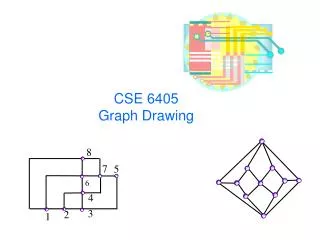
Straight line drawings of planar graphs – part I. Roeland Luitwieler. Outline. Introduction The shift method The canonical ordering The shift algorithm Next time: the realizer method. Introduction. This presentation is about: Straight line grid drawings of planar graphs Minimized area

E N D
Straight line drawings of planar graphs – part I Roeland Luitwieler
Outline • Introduction • The shift method • The canonical ordering • The shift algorithm • Next time: the realizer method
Introduction • This presentation is about: • Straight line grid drawings of planar graphs • Minimized area • De Fraysseix, Pach & Pollack, 1988: • The shift method: 2n–4 x n–2 grid • Schnyder, 1990: • The realizer method: n–2 x n–2 grid • Both are quite different, but can be implemented as linear time algorithms
Introduction • Assumptions (can be taken care of in linear time) • n ≥ 3 (trivial otherwise) • Graph is maximal planar (=triangulated) • Graph has a topological embedding • Terminology • Given an ordering on the vertices of graph G: • Gk is the induced subgraph of vertices v1, …, vk • Co(G) is the outer cycle of a 2-connected graph G • Given a cycle C with u and v on it, but (u,v) not on it: • The edge (u,v) is a chord of C
The canonical ordering • An ordering of vertices v1, …, vn is canonical if for each index k, 3 ≤ k ≤ n: • Gk is 2-connected and internally triangulated • (v1, v2) is on Co(Gk) • If k+1≤n, vk+1 is in the exterior face of Gk and its neighbours in Gk appear on Co(Gk) consecutively
The canonical ordering • Lemma: every triangulated plane graph has a canonical ordering • Trivial for n=3, so assume n≥4 • Proof by reverse induction • Base case (k=n): conditions hold since Gn = G • Co(Gn) consists of v1, v2 and vn • We now assume that vn, vn-1, ..., vk+1 for k+1≥4 have been appropriately chosen and that the conditions hold for k • To prove: the conditions hold for k–1
The canonical ordering • If we can find a vertex (= vk) on Co(Gk) which is not an end of a chord, the conditions hold • Follows from Gk–1 = Gk – vk • Such a vertex always exists, because a chord always skips at least one vertex on the cycle
The canonical ordering • A canonical ordering of a triangulated plane graph can be found in linear time • Use labels for vertices • Label -1 means not yet visited • Label 0 means visited once • Label i means visited more than once and there are i intervals of visited neighbours in the circular order around the vertex • Algorithm: • Let v1 and v2 be two consecutive vertices on Co(G) in counter clockwise order • Label all other vertices -1 • Process v1 • Process v2 • for k = 3 to n do • Chose a vertex v with label 1 • vk = v • Process vk
The canonical ordering • (Sub-algorithm) Process v: • For all neighbours w of v not yet processed do • If label -1 then label(w) = 0 • If label 0 then (w has one processed neighbour u) • If w next to u in circular order of neighbours of v then label(w) = 1 • Otherwise label(w) = 2 • Otherwise (label i) • If vertices next to w in circular order of neighbours of v both have been processed then label(w) = i–1 • If neither has been processed yet then label(w) = i+1 • Correctness • All processed vertices form Gk and the chosen vertex is vk+1 • Verify the conditions hold now • Successful termination guaranteed by previous proof
The shift algorithm • General idea: • Insert vertices in canonical order in drawing • Invariants when inserting vk: • x(v1) = 0, y(v1) = 0, x(v2) = 2k–6, y(v2) = 0 • x(w1) < … < x(wt) where Co(Gk–1) = w1, …, wt with w1 = v1, wt = v2 • Each edge on Co(Gk–1) except (v1, v2) is drawn by a straight line having slope +1 or –1
The shift algorithm • General idea: • Some vertices need to be shifted when inserting vk
The shift algorithm • To obtain a linear time algorithm, x-offsets are used in stead of x-coordinates • We use a binary tree to represent shift dependencies • Each node shifts whenever its parent shifts • Store x-offset and y-coordinate in each node • Using the tree, the x-offsets can be accumulated in linear time
The shift algorithm • Compute x-offsets and y-coordinates: • Compute values and create the tree for G3 • For k = 4 to n do • Let w1, …, wt = Co(Gk–1) with w1 = v1, wt = v2 • Let wp, wp+1, …, wq be the neighbours of vk on Co(Gk–1) • Increase Δx(wp+1) and Δx(wq) by one • Compute Δx(vk) and y(vk) • Update the tree accordingly
The shift algorithm • Updating the tree
The shift algorithm • Computing Δx(vk) and y(vk) • Δx(wp, wq) = Δx(wp+1) + ... + Δx(wq) • Δx(vk) = ½ {Δx(wp, wq) + y(wq) – y(wp)} • y(vk) = ½ {Δx(wp, wq) + y(wq) + y(wp)} • Other necessary updates: • Δx(wq) = Δx(wp, wq) – Δx(vk) • If p+1 <> q then Δx(wp+1) = Δx(wp+1) – Δx(vk)
Conclusions • The shift method uses • The canonical ordering • A 2n–4 x n–2 grid, obviously • Linear time • Next time: the realizer method • Questions?
References • H. de Fraysseix, J. Pach and R. Pollack, How to draw a planar graph on a grid, Combinatorica 10 (1), 1990, pp. 41–51. • D. Harel and M. Sardas, An Algorithm for Straight-Line Drawing of Planar Graphs, Algorithmica 20, 1998, pp. 119–135. • T. Nishizeki and Md. S. Rahman, Planar Graph Drawing, World Scientific, Singapore, 2004, pp. 45–88. • W. Schnyder, Embedding planar graphs on the grid, in: Proceedings of the First ACM-SIAM Symposium on Discrete Algorithms, 1990, pp. 138–148.