QuickSort Algorithm
QuickSort Algorithm. Using Divide and Conquer for Sorting. Topics Covered . QuickSort algorithm analysis Randomized Quick Sort A Lower Bound on Comparison-Based Sorting. Quick Sort. Divide and conquer idea: Divide problem into two smaller sorting problems. Divide:

QuickSort Algorithm
E N D
Presentation Transcript
QuickSort Algorithm Using Divide and Conquer for Sorting
Topics Covered • QuickSort algorithm • analysis • Randomized Quick Sort • A Lower Bound on Comparison-Based Sorting
Quick Sort • Divide and conquer idea: Divide problem into two smaller sorting problems. • Divide: • Select a splitting element (pivot) • Rearrange the array (sequence/list)
Quick Sort • Result: • All elements to the left of pivot are smaller or equal than pivot, and • All elements to the right of pivot are greater or equal than pivot • pivot in correct place in sorted array/list • Need: Clever split procedure (Hoare)
Quick Sort Divide: Partition into subarrays (sub-lists) Conquer: Recursively sort 2 subarrays Combine: Trivial
QuickSort (Hoare 1962) Problem: Sort n keys in nondecreasing order Inputs: Positive integer n, array of keys S indexed from 1 to n Output: The array S containing the keys in nondecreasing order.quicksort ( low, high )1. if high > low2. then partition(low, high, pivotIndex)3. quicksort(low, pivotIndex -1)4. quicksort(pivotIndex +1, high)
Partition array for Quicksort partition (low, high, pivot)1. pivotitem = S [low]2. k = low3. for j = low +1 to high4. do if S [ j ] < pivotitem5. then k = k + 16. exchange S [ j ] and S [ k ] 7. pivot = k8. exchange S[low] and S[pivot]
5 3 6 2 5 3 6 2 5 3 6 2 after line3 k j k j k j 5 3 6 2 after line5 5 3 6 2 j,k k j 5 3 2 6 after line6 5 3 6 2 k j j,k pivot k Input low =1, high = 4pivotitem = S[1]= 5 after loop 5 3 2 6
k j Partition on a sorted list 3 4 6 3 4 6 after line3 k j after loop 3 4 6 pivotk How does partition work for S = 7,5,3,1 ?S= 4,2,3,1,6,7,5
Worst Case Call Tree (N=4) Q(1,4) S =[ 1,3,5,7 ] Left=1, pivotitem = 1, Right =4 Q(2,4) Left =2,pivotItem=3 Q(1,0) S =[ 3,5,7 ] Q(2,1) Q(3,4)pivotItem = 5, Left = 3 S =[ 5,7 ] Q(4,4) S =[ 7 ] Q(3,2) Q(5,4) Q(4,3)
n å k = 1 0 0 Worst Case Intuition n-1 n-1 t(n) = n-2 n-2 0 n-3 n-3 0 n-4 n-4 0 . . . 1 1 0 Total = k = (n+1)n/2 0
n/8 n/8 n/8 n/8 ..> ..> Recursion Tree for Best Case Partition Comparisons n n Nodes contain problem size n n/2 n/2 n/4 n/4 n/4 n/4 n n/8 n/8 n n/8 n/8 ..> ..> Sum =(n lgn)
Another Example of O(n lg n) Comparisons • Assume each application of partition () partitions the list so that (n/9) elements remain on the left side of the pivot and (8n/9) elements remain on the right side of the pivot. • We will show that the longest path of calls to Quicksort is proportional to lgn and not n • The longest path has k+1 calls to Quicksort= 1 + log 9/8n 1 + lgn / lg (9/8) = 1 + 6lgn • Let n = 1,000,000. The longest path has1 + 6lgn = 1 + 620 = 121 << 1,000,000calls to Quicksort. • Note: best case is 1+ lgn = 1 +7 =8
256n/729 ..> ..> ..> Recursion Tree for Magic pivot function that Partitions a “list” into 1/9 and 8/9 “lists” n n n/9 n 8n/9 n (log9n) n/81 8n/81 8n/81 64n/81 (log9/8n) n/729 9n/729 ..> n 0/1 ... <n 0/1 0/1 <n 0/1
n 1 n-1 (n-1)/2 (n-1)/2 Intuition for the Average caseworst partition followed by the best partition Vs n 1+(n-1)/2 (n-1)/2 This shows a bad split can be “absorbed” by a good split. Therefore we feel running time for the average case is O(n lg n)
T(n) = max ( T(q-1) + T(n - q) )+ Q (n) 0 £ q£ n-1 Recurrence equation: Worst case Average case n A(n) = (1/n) å (A(q -1) + A(n - q ) ) + Q (n) q = 1
Sorts and extra memory • When a sorting algorithm does not require more than Q(1) extra memory we say that the algorithm sorts in-place. • The textbook implementation of Mergesort requires Q(n) extra space • The textbook implementation of Heapsort is in-place. • Our implement of Quick-Sort is in-place except for the stack.
Quicksort - enhancements • Choose “good” pivot (random, or mid value between first, last and middle) • When remaining array small use insertion sort
Randomized algorithms • Uses a randomizer (such as a random number generator) • Some of the decisions made in the algorithm are based on the outputoftherandomizer • The output of a randomized algorithm couldchange from run to run for the same input • The executiontime of the algorithm could also vary from run to run for the same input
Randomized Quicksort • Choose the pivot randomly (or randomly permute the input array before sorting). • The running time of the algorithm is independent of input ordering. • No specific input elicits worst case behavior. • The worst case depends on the random number generator. • We assume a random number generator Random. A call to Random(a, b) returns a random number between a and b.
RQuicksort-main procedure // S is an instance "array/sequence" // terminate recursionquicksort ( low, high )1. if high > low2a. then i=random(low, high); 2b. swap(S[high], S[I]); 2c. partition(low, high, pivotIndex)3. quicksort(low, pivotIndex -1)4. quicksort(pivotIndex +1, high)
Randomized Quicksort Analysis • We assume that all elements are distinct (to make analysis simpler). • We partition around a random element, all partitions from 0:n-1 to n-1:0 are equally likely • Probability of each partition is 1/n.
Summary of Worst Case Runtime • exchange/insertion/selection sort = Q(n 2) • mergesort = Q(n lg n ) • quicksort = Q(n 2 ) • average case quicksort = Q(n lg n ) • heapsort = Q(n lg n )
Sorting • So far, our best sorting algorithms can run inQ(n lg n) in the worst case. • CAN WE DO BETTER??
Goal • Show that any correct sorting algorithm based only on comparison of keys needs at least nlgn comparisons in the worst case. • Note: There is a linear general sorting algorithm that does arithmetic on keys. (not based on comparisons) Outline: 1) Representing a sorting algorithm with a decision tree. 2) Cover the properties of these decision trees. 3) Prove that any correct sorting algorithm based on comparisons needs at least nlgn comparisons.
Decision Trees • A decision tree is a way to represent the working of an algorithm on all possible data of a given size. • There are different decision trees for each algorithm. • There is one tree for each input size n. • Each internal node contains a test of some sort on the data. • Each leaf contains an output. • This will model only the comparisons and will ignore all other aspects of the algorithm.
For a particular sorting algorithm • One decision tree for each input size n. • We can view the tree paths as an unwinding of actual execution of the algorithm. • It is a tree of all possible execution traces.
if a < b then if b < c then S is a,b,celse if a < c then S is a,c,belse S is c,a,b else if b < c thenif a < c then S is b,a,celse S is b,c,a else S is c,b,a sortThree a<- S[1]; b<- S[2]; c<- S[3] a<b yes no b<c b<c yes no yes no a,b,c a<c c,b,a a<c yes yes no no b,a,c c,a,b a,c,b b,c,a Decision tree for sortThree Note: 3! leaves representing 6 permutations of 3 distinct numbers. 2 paths with 2 comparisons 4 paths with 3 comparisons total 5 comparison
1. for (i = 1; i n -1; i++)2. for (j = i + 1; j n ; j++)3. if ( S[ j ] < S[ i ])4. swap(S[ i ] ,S[ j ]) Exchange Sort At end of i = 1 : S[1] = minS[i] At end of i = 2 : S[2] = minS[i] At end of i = 3 : S[3] = minS[i] 1 i n 2 i n n- 1 i n
c,b,a a,b,c Decision Tree for Exchange Sort for N=3 Example =(7,3,5) a,b,c s[2]<s[1] i=1 3 7 5 b,a,c a,b,c ab s[3]<s[1] s[3]<s[1] 3 7 5 b,a,c c,b,a a,b,c c,a,b cb ca s[3]<s[2] s[3]<s[2] s[3]<s[2] s[3]<s[2] cb ca ab ab b,c,a c,a,b a,c,b c,a,b c,b,a b,a,c 3 5 7 Every path and 3 comparisonsTotal 7 comparisons8 leaves ((c,b,a) and (c,a,b) appear twice.
Questions about the Decision TreeFor a Correct Sorting Algorithm Based ONLY on Comparison of Keys • What is the length of longest path in an insertion sort decision tree? merge sort decision tree? • How many different permutation of a sequence of n elements are there? • How many leaves must a decision tree for a correct sorting algorithm have? • Number of leaves n ! • What does it mean if there are more than n! leaves?
Proposition: Any decision tree that sorts n elements has depth (n lg n ). • Consider a decision tree for the best sorting algorithm (based on comparison). • It has exactly n! leaves. If it had more than n! leaves then there would be more than one path from the root to a particular permutation. So you can find a better algorithm with n! leaves. • We will show there is a path from the root to a leaf in the decision tree with nlgn comparisonnodes. • The best sorting algorithm will have the "shallowest tree"
Proposition: Any Decision Tree that Sorts n Elements has Depth (n lg n ). • Depth of root is 0 • Assume that the depth of the "shallowest tree" is d (i.e. there are d comparisons on the longest from the root to a leaf ). • A binary tree of depth d can have at most 2dleaves. • Thus we have : n! 2d,, taking lg of both sides we get d lg (n!). It can be shown that lg (n !) = (n lg n ). QED
Implications • The running time of any whole key-comparison based algorithm for sorting an n-element sequence is (n lg n ) in the worst case. • Are there other kinds of sorting algorithms that can run asymptotically faster than comparison based algorithms?