Download

1 / 34
350 likes | 580 Vues
CENSORED MATERIAL!!!. 600 Down: What’s Up with IceCube?. Status and Future of the IceCube Neutrino Observatory Kael Hanson for the IceCube Collaboration TeV Particle Astrophysics II Madison, WI August 28-31, 2006. The AMANDA/IceCube Authors. Physics Motivations for TeV Neutrino Observatory.

E N D
CENSORED MATERIAL!!! 600 Down: What’s Up with IceCube? Status and Future of the IceCube Neutrino Observatory Kael Hanson for the IceCube Collaboration TeV Particle Astrophysics II Madison, WI August 28-31, 2006
Physics Motivations for TeV Neutrino Observatory • Search for cosmic-ray accelerators • Active galactic nuclei • Supernova remnants • Gamma-ray bursts • Neutrinos are ideal messenger – carry information from potentially deep within a source pointing back to it • Protons except for EHE are bent in magnetic fields. • EHE protons interaction on CMBR (GZK cutoff) • HE photons are absorbed by interaction with CMBR • Neutrinos are guaranteed via “beam-dump” production mechanism. • Cross-section very small – build km-scale observatories. Figure byP. Gorham • Neutrino / particle-physics (105 atmnu/year!): • UHE cross-section measurements • Charm physics • Neutrino oscillations • Tests Lorentz Invariance – gamma of TeV-scale neutrinos way beyond reach of other techniques. • Supersymmetry / WIMPs, exotic particles • Supernova neutrinos (MeV-scale)
AMANDA • 677 analog OMs deployed along 19 strings • 10 strings 1997 (AMANDA B10) • 3 strings 1998 (AMANDA B13) • 6 strings 2000 (AMANDA II) • Analog PMT signals using electrical and optical transmission lines. • 200 m diameter, 500 meters height; AMANDA II encompasses 20 Mton instrumented ice volume. • AMANDA will remain operational and form IceCube Inner Core Detector for low E physics (~ 100 GeV) • IceCube surrounding strings provide effective veto – lower background and can push AMANDA energy threshold down. • Conventional TDC / ADC technology for AMANDA has been entirely replaced by TWR system. • Beginning 2007 season, AMANDA / IceCube data streams will be conjoined; detector subsystems will share trigger information.
AMANDA Atmospheric Neutrinos / Diffuse Flux Limit Limit on diffuse E-2νμflux (100-300 TeV): E2μ(E) < 2.6·10–7 GeV cm-2 s-1 sr-1 Includes 33% systematic uncertainty
AMANDA Skymap Significance / s 2000-2004 Largest fluctuation: 3.7s at 12.6 h, +4.5 deg Random events 69 out of 100 sky maps with randomized events show an excess higher than 3.7s No significant “hot spot”
The IceCube Detector Array Design Specifications • Fully digital detector concept. • Number of strings – 75 • Number of surface tanks – 160 • Number of DOMs – 4820 • Instrumented volume – 1 km3 • Muon effective area – see plot • Angular resolution of in-ice array < 1.0° Current Status • 9 strings, 16 surface stations • 604 deployed DOMs, 594 taking data (98%) • Instrumented volume ~ 0.1 km3 • Collecting physics data
IceCube effective area and angular resolution for muons Galactic center further improvement expected using waveform info • E-2νμ spectrum • quality cuts and background suppression (atm μ reduction by ~106) Median angular reconstruction uncertainty ~ 0.8
Point Sources and Diffuse Fluxes in the IceCube Era * AMANDA-B10 average flux upper limit [cm-2s-1] AMANDA-II IceCube 1/2 year sin(d)
Cosmic Ray Physics : IceCube Deep-Ice Array + IceTop Deep-ice array + IceTop form 3D airshower detector with 0.3 km2·sr acceptance – very powerful combination for cosmic ray physics. South Pole altitude near shower max for 10 PeV primaries – almost perfect placement from standpoint of minimizing fluctuations in “knee” region of CR spectrum. Energy Mass Fig. by R. Engel As shown in plot above Z, ECR by simultaneous measurement of deep-ice detector response (Nμ) and surface array (Ne). SPASE-AMANDA published result:Astropart. Phys. 21 (565)
2005, 2006, 2007 Deployments AMANDA 80 79 IceCube string and IceTop station deployed 01/05 74 73 72 67 66 65 IceCube string and IceTop station deployed 12/05 – 01/06 59 58 57 56 50 49 48 47 IceTop station only 2006 46 40 39 38 IceCube string and IceTop station to be deployed 12/06 – 01/07 30 29 21 604 DOMs deployed to date Next year looking for ≥ 12 strings. IceTop will be backed off to remain in line with hole deployment Want to achieve steady state of 14 strings / season.
IceCube Integrated Volume (Projected) • Graph shows cumulative km3·yr of exposure × volume • # of strings per year is based on latest “best guess” deployment rate of 12 strings next year and 14 strings per season thereafter. • 1 km3·yr reached 2 years before detector is completed • Close to 4 km3·yr at the beginning of 2nd year of full array operation.
Finding neutrinos in the ice Point-like cascades νe CC or νX NC nuclear interactions produce either EM or hadronic cascades. These cascades can produce enormous amounts of Cherenkov photons (108 photons per TeV) which are radiated over 4π. The extent of the particle cascade is small; the expanding, approximately spherical wavefront appears to come from a point. Eµ=10 TeV ~300m for >PeV t Track-like muons νμ (or VHE μτ) in CC interaction with nucleus will produce outgoing μ or τ which radiates Cherenkov photons in conical wavefront expanding outward from linear track. Typically the interaction vertex lies outside the fiducial detector volume (through-going event) and only track is seen. However, hadronic cascade from recoiling target inside contained volume is also possible. “Double-bang” VHE ντ interacting inside the detector produces the primary recoil cascade and a τ which radiates as muon tracks until it decays and produces a secondary cascade – leaving a very distinct event signature.
Ice Properties Why deploy in ice? Deep glacial ice is optically transparent. Two mechanisms: scattering length ~ 20 m, absorption ~ O(100) m. Ice has several layers of dust from prehistoric events. Monte Carlo detector simulation must account for this. Reconstruction methods involving maximum likelihood tests against hypotheses have been developed to overcome difficulties posed by photon scattering. Plots above from in situ measurements using artificial light sources in AMANDA. “Hole ice” around deployed modules must also be taken into account.
The Enhanced Hot Water Drill (EHWD) EHWD designed to drill a 2450 m × 60 cm hole in ~30 hr. Fuel budget is 7200 gal per hole. Shown above is drill camp and tower site (inset), both mobile field arrays. Everything must fit into LC-130 for transport to Pole. Supply: 200 GPM @ 1000 psi, 190 °FReturn: 192 GPM @ 33 °F Make-Up: 8 GPM @ 33 °F Thermal Power: 4.5 Megawatt
Drilling Ted Schultz Top layer of packed snow is called firn. Hot water drill designed for ice drilling – it gets starter hole from firn drill (lower right). (Top left and top right) EHWD drill head entering hole.
IceCube DOM DOM Requirements • Fast timing: resolution < 5 ns DOM-to-DOM on LE time. • Pulse resolution < 10 ns • Optical sens. 330 nm to 500 nm • Dynamic range - 1000 pe / 10 ns - 10,000 pe / 1 us. • Low noise: < 500 Hz background • High gain: O(107) PMT • Charge resolution: P/V > 2 • Low power: 3.75 W • Ability to self-calibrate • Field-programmable HV generated internal to unit. • Flasher board – capable of emitting optical pulses O(20) ns wide > 109 γ/pulse • 10000 psi external
DOM Production – DOM Assembly 1. PMT prepared by gluing plastic collar to hold board stack – HV base soldered onto leads DOMs Shipped to Pole 2. Bottom hemisphere holds magnetic shield and RTV gel – mechanical interface to PMT 3. PMT potted in gel – held to precision location by potting jig 4. Board stack mounted onto PMT collar 5. Top hemisphere / penetrator cable soldered onto mainboard. 6. Sphere brought down to 0.5 atm and taped.
Preliminary Detector Performance In-Ice Verification activity ongoing this year to check proper operation of IceCube at higher level. Time resolution is vital detector performance parameter: checks of this quantity at advanced stage – all indicating DOM-to-DOM time resolution is better than 5 ns. rms time resolution of DOMs on string 21 from flasher data. Muon Occupancy plot which shows fraction of times given DOM produced hit when it’s string was hit. Structure is primarily due to (z-dep) dust layers (cf. ice optics slide) Plot demonstrating the timing residual from tracks reconstructed using the 9-string detector.
Data Acquisition DOM Mainboard This is the guts of the DAQ. It contains an Altera Excalibur ARM CPU / 400 k-gate FPGA which controls most aspects of the acquisition and communications with the surface. All aspects except bootloader program remotely reloadable. Fast waveform capture via 1 of 2 ATWD ASICs which capture 4 ch at 200 MSPS – 800 MSPS, 128 samples deep and 10-bits wide. ATWDs operate in “ping-pong” mode – true deadtimeless operation possible. 3 ch are high, medium, low gain (14-bit effective dynamic range). Slow waveform capture from 40 MHz 10-bit FADC which captures long slow pulses for 6.4 usec. Digital communication to surface using electrical pairs – two DOMs per pair. Electrical penetrators more robust. Communication bandwidth 1 Mbit. DOM contains local free-running oscillator. DOM – DOM clock synchronization via RAPCal mechanism which involves exchange of analog pulses from surface to DOM and back to surface. This coordinates local clock with global surface clocks slaved to GPS-driven master. The power of a digital system which automatically calibrates itself was appreciated when we first turned on the strings and tanks and immediately analysis-ready data was flowing from the DOMs. DFL measurements (easy – synchronous source) and measurements in the ice (harder – no synchronous source) along real cable indicate precision of RAPCal mechanism is better than 2.5 ns.
Surface DAQ • DOMs independently collect and buffer up to 8k waveforms. • DOM communication handled at surface by DOR card – hosted by standard industrial PCs called ‘DOMHub.’ • Beyond Linux driver DAQ software is a distributed set of Java applications. • Data is time coordinated and sorted by processing nodes which may in future perform data reduction. • Triggers take sorted streams; request to event builder to grab data from string processors and IceTop data handlers to make events. • Note: data from deep-ice and surface arrays participate in triggers and are bundled together at event level. • Online filter at pole selects ‘interesting’ events for transmission north over satellite (limited bandwidth). • All data taped – raw data rate currently 70 GB / day.
Triggers and Events • DAQ operational since station close – Feb 13, 2006. As of 8/26 1.5×10⁹ events collected. • Triggers formed in application software – pluggable framework exists for creation of new triggers. Configuration framework allows run-time programming of trigger parameters. • Current triggers in use are • SMT : Simple Majority Trigger triggers on 8-fold coincidence in 5 μs window (in-ice array); 6-fold coincidence in 5 μs (IceTop). • MBT : Minimum Bias Trigger selects every 1000th hit. • Global Trigger process decides whether sub-detector triggers actually trigger detector, possibly merges several overlapping triggers, and sends trigger request to Event Builder. • EventBuilder collects hits around triggers (± 8μs) and forms event structure.
Local Coincidence Modes 1 1 1 1 2 2 2 2 3 3 3 3 4 4 4 4 5 5 5 5 DOMs contain 2 wire pair (UP, DN) for exchanging LC signals between adjacent DOMs on string†. DOM FPGA trigger logic can abort waveform capture on absence of one or both signals. LC signals are binary-coded digital – DOMs can “relay” LC info thru; in this manner LC can span up to 4 DOMs distant in either direction. IceCube currently running in NN mode – that is DOM trigger requires adjacent hit (red circles) – as shown in case A to right. In this mode B and D would not trigger, C would trigger only 1 and 2 and reject 4. This has advantage of (a) dramatically reducing amount of data sent over 1 Mbit link to surface (see figure) and (b) makes array virtually “noiseless.” Disadvantage is that real photon hits are lost in ice. IceCube baseline – operate in “soft” LC mode: waveforms suppressed /wo/ LC requirement, all hit timestamps (12 bytes) sent to surface. A B C D †(IceTop configured so that UP/DN neighbors are 2 DOMs in conjugate station).
IceCube Events IceTop /w/ Reco Neutrino Candidate Joint IceTop-InIce
Outlook • Experience from last year: • Drill system capable of producing 2 holes per week • Digital optical module is manufacturable in large quantities and is robust: of 604 DOMs in or on the ice – 594 taking data. • IceCube array is operational with 9 strings and collecting ~ 150 ev/sec. Preliminary online data filter extracting candidate atmospheric neutrino events. • Preliminary indications from timing data checks are that DOM performance meets or exceeds spec. • String deployment plan: 12 strings next year (logistics support for 14), then 14 each year thereafter. Looking to reach target of ~75 strings. • IceCube will reach 1 km2∙yr Feb 2009, well before the actual completion date in 2011. • South Pole ice good medium for non-optical detection techniques acoustic and radio. IceCube likely to become inner core detector for 100 km2 array.
The End Overflow slides
ATWD Waveforms • Pulse shapes are recorded with three ATWD channels for high dynamic range coverage. • Runs of 10 flasherboard pulses at 5 different brightness settings are shown. • High saturation in channel 0 (high gain), but good coverage of the brightest pulses in channel 2 (low gain). • ATWD has excellent time resolution (300 MHz typ. sample speed) and dynamic range coverage – however longer time windows must be captured using 40 MHz FADC.
Importance of noise rates: 1.) noise rate w/o dead time: 700 Hz, important for DAQ bandwidth 2.) noise rate w/suppression of 50µs: 300Hz, important for event reconstruction and in particular for supernova sensitivity. Two Icecube strings equivalent or more sensitive than all of AMANDA to SN.
DOMCal • Monthly calibration of DOM • Process takes approx 1 hour, can be administered from NH • Front-end amplifier, discriminator, and digitizer chip calibrations, PMT gain versus HV mapping, and PMT transit time. • All computations – including non-linear minimization – executed on DOM ARM CPU! • Results stored on DOM flash filesystem • Results also uploaded from DOM for permanent storage in XML files and SQL database 1180 VDC 1260 VDC 1340 VDC 1420 VDC 1500 VDC 1580 VDC 1660 VDC 1740 VDC 1820 VDC Gain(HV) Fit