Download
1 / 32
320 likes | 462 Vues
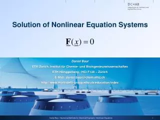
Solution of Nonlinear Equation (b). Dr. Asaf Varol asvarol@mail.wvu.edu. Secant Method. Similar approach as the Newton-Raphson method Differs because the derivative does not need to be calculated analytically, which can be a great advantage F (x i ) = [F(x i ) - F(x i-1 )]/(x i – x i-1 )

E N D
Solution of Nonlinear Equation (b) Dr. Asaf Varol asvarol@mail.wvu.edu
Secant Method • Similar approach as the Newton-Raphson method • Differs because the derivative does not need to be calculated analytically, which can be a great advantage F(xi) = [F(xi) - F(xi-1)]/(xi – xi-1) • Disadvantage is that two initial guesses are needed instead of one
Graphical Interpretation of Newton-Raphson and Secant Method
Example: Secant Method • Water flow from a tower at a height h, through a pipe of diameter D and length L which is connected to the tower running vertically downward and then laid horizontally to the desired point of delivery. For this system the following equation for the flow rate Q is found. Find the roots using the Secant Method.
Multiplicity of Roots and Newton-Based Methods • In some situations, one root can fulfill the role of being a root more than one time. For example, the equation F(x) = x3 - x2 - x + 1= (x + 1)(x - 1)2 = 0 has three roots, namely x = -1, and x = 1 with a multiplicity of two • Using l’Hospital’s Rule, the Newton-Raphson method can be modified xi+1 = xi - F(xi)/F(xi) Or, if the second derivative is also zero then l'Hospital's rule can be applied once more to obtain xi+1 = xi - F(xi)/F(xi)
Example E2.4.1 Problem: Apply Newton-Raphson method to the polynomial equation F(x) = x3 - 3x2 + 3x - 1 = (x - 1)3 = 0 Solution: First we apply Newton-Raphson method without any modification of the given function. It can be shown that the method does not converge for any of the starting values x0 = 0., 0.5, 0.9, and 1.5. In fact the iterations oscillate between 0.2504306 and 0.4258722. But if we make the following substitution U(x) = F(x) and U(x) = F(x) and apply the same method, i.e. xi+1 = xi - U(xi)/U(xi) then the method converges in 24 iterations to the root x=.9999999 with an error bound of 1.0E-07, and starting value of x=0.0
Systems of Nonlinear Equations • Extension of the previous methods to systems of N equations with N variables • Our discussion will be limited to solutions to the following system of nonlinear equations: F(x,y) = 0 G(x,y) = 0 • For example, x2 + y2 - 2 = 0 -exp(-x) + y2 - 1 = 0
Jacobi Iteration Method • Jacobi method is an extension of the fixed-point iteration method to systems of equations • The equations F(x,y) = 0 G(x,y) = 0 need to be transformed into x = f(x,y) y = g(x,y) • Actual iteration is similar to the case of one equation with one variable xi+1 = f(xi,yi) yi+1 = g(xi,yi)
Jacobi Iteration Method • Convergence criteria - in the vicinity of the root (xr, yr),
Matlab for Jacobi Method • %Jacobi Iteration Method • x0=0.0; • y0=0.0 • E=1.0E-4; • % • %---writing out headers to the file 'jacobimethod.dat' • % • fid=fopen('jacobi.dat','w'); • fprintf(fid,'Roots of Equations x-5+exp(-xy)=0 \n\n') • fprintf(fid,'Roots of Equations y-1+exp(-0.5x)cos(xy)=0 \n\n') • fprintf(fid,'Using Jacobi Method \n') • fprintf(fid,'iter x y ErrorX ErrorY \n'); • fprintf(fid,'------------------------------------------\n'); • % • %---entering the loop to determine the root • %
Matlab for Jacobi Method (Cont’d) • for i=1:100 • x1=5-exp(-x0*y0); • y1=1-exp(-0.5*x0)*cos(x0*y0); • errorx=abs(x1-x0); • errory=abs(y1-y0); • %---writing out results to the file 'jacobi method.dat' • % • fprintf(fid,'%4.1f %7.4f %7.4f %7.4f %7.4f \n',i,x1,y1,errorx,errory); • % • if abs(x1-x0)<E&abs(y1-y0)<E • break; • end • x0=x1; • y0=y1; • end • fclose(fid) • disp('Roots approximation=') • x1,y1
Gauss-Seidel Iteration Method • Similar to the Jacobi iteration method • Differs by using updated x or y values (i.e. the approximate roots) for calculations
Newton’s Method (I) • Consider the two nonlinear equations F(x,y) = 0 G(x,y) = 0 • The Taylor series expansion for a function F(x, y) is where ( )x and ( )xx denote the first and second partial derivatives with respect to x, and similarly for ( )y , ( )yy and ( )xy
Newton’s Method (II) • Keeping the first three terms on the right-hand side yields • Solving these equations for x and y after letting yields where J is the Jacobian defined by J = (FxGy - GxFy)
Newton’s Method (III) • Retaining only two terms and thus simplifying the equations,
Technique of Underrelaxation and Overrelaxation • Expresses ‘confidence’ in the new estimate of the root • Underrelaxation 0 < < 1 • Overrelaxation - 1 < < 2 • Can be applied to Newton’s method as
Case Study C2.3: Damped Oscillation of an Object (continued)
Case Study C2.3: Damped Oscillation of an Object (continued)
Case Study C2.3: Damped Oscillation of an Object (continued)
Case Study C2.3: Damped Oscillation of an Object (continued)
Case Study C2.3: Damped Oscillation of an Object (continued)
Case Study C2.3: Damped Oscillation of an Object (continued)
References • Celik, Ismail, B., “Introductory Numerical Methods for Engineering Applications”, Ararat Books & Publishing, LCC., Morgantown, 2001 • Fausett, Laurene, V. “Numerical Methods, Algorithms and Applications”, Prentice Hall, 2003 by Pearson Education, Inc., Upper Saddle River, NJ 07458 • Rao, Singiresu, S., “Applied Numerical Methods for Engineers and Scientists, 2002 Prentice Hall, Upper Saddle River, NJ 07458 • Mathews, John, H.; Fink, Kurtis, D., “Numerical Methods Using MATLAB” Fourth Edition, 2004 Prentice Hall, Upper Saddle River, NJ 07458 • Varol, A., “Sayisal Analiz (Numerical Analysis), in Turkish, Course notes, Firat University, 2001