Example 9
Example 9. Design Storms in HEC-HMS. Purpose. Illustrate the steps to create a design storm in HEC-HMS. The example will create a variety of design storms for a particular Texas location.

Example 9
E N D
Presentation Transcript
Example 9 Design Storms in HEC-HMS
Purpose • Illustrate the steps to create a design storm in HEC-HMS. • The example will create a variety of design storms for a particular Texas location. • Focus on HOW to construct the hyetograph (for design storms requiring external processing) and the two built-in methods
Learning Objectives • Generate an input hyetograph design storm using several different methods. • External processed storms • Generate an SCS and Frequency Storm using HEC HMS • Internal processed storms • Generate rapid generic HMS models for creating input data (for later export).
Problem Statement • Generate a 24-hour, 25-year design storm for Harris Co. Texas using • SCS Design Storm Approach and EBDLKUP • 0-4194-3 Empirical Hyetograph • Generate a 6-hour, 25-year design storm for Harris Co. Texas using • SCS Design Storm Approach and EBDLKUP • 0-4194-3 Empirical Hyetograph
Problem Statement • Generate a 24-hour, 25-year design storm for Harris Co. Texas using • Frequency Storm and DDF Atlas
Required Tools • TP-40, HY35, DDF Atlas, or EBDLKUP • This example will use both the DDF Atlas and EBDLKUP to illustrate use of the two tools, you don’t need both. • 0-4194-3 Empirical Hyetographs
Precipitation Depth • Using EBDLKUP • 24 hr, 25 yr Depth = 10.01 inches • 6 hr, 25 yr Depth = 6.75 inches
Rapid HMS Model • Create a new project • Basin model • Dummy subbasin • No loss • No UH transform
Rapid HMS Model • Create a new project • Meterological model • SCS Storm
Rapid HMS Model • Meterological model • SCS Storm • Select Type • Insert Depth
Rapid HMS Model • Control Specifications • Time Window • 24 hours for SCS storm
Rapid HMS Model • Run the model
Rapid HMS Model • We will want the SCS 24-hour storm for the later work, so lets get a copy from HMS. • Observe that element time series has no rain – storm is produced directly, but we can convert the 1 sq.mi. discharge into watershed inches/hour in Excel
HEC-HMS Output • Convert the No-transform hydrograph into the SCS Type 2 storm (AREA=1 sq. mi.)
6-Hour Storm • Now we will figure out the 6 hour SCS storm. • Idea is to use the most intense part of the storm. • Use the 6 hours centered on 12:00 of the storm, rescale these to the correct depth and we have a 6-hour storm.
SCS 6-hour, Unscaled • Pick the 6-hour period. • Then set remainder to zero • Compute total depth • Adjust to get the required total depth of 6.75 inches
SCS 6-hour, Unscaled • Pick the 6-hour period. • Then set remainder to zero • Compute total depth • Adjust to get the required total depth of 6.75 inches
SCS 6-hour, Unscaled • Pick the 6-hour period. • Then set remainder to zero • Compute total depth • Adjust to get the required total depth of 6.75 inches
SCS 6-hour, Scaled • Pick the 6-hour period. • Then set remainder to zero • Compute total depth • Adjust to get the required total depth of 6.75 inches
SCS 6-hour, Scaled • Cut and past into HMS • Time series data manager
HEC-HMS Model • Run the model
HEC-HMS Model • Summary • SCS 24-hr is “built-in”, specify storm type and depth. • SCS 6-hr is processed externally • Results • 24 hr, Qp = 9340 cfs, Tp = 11:52 , V= 10.01 in. • 6 hr, Qp = 8905 cfs , Tp = 2:52 , V = 6.75 in • Recall the Qp are not true “runoff” in this example – they represent “excess precipitation” expressed in units of watershed discharge for a 1 sq. mi. watershed.
Using DDF Atlas • Repeat the example using the DDF atlas • Need two maps; 25 yr – 24 hr and 25 yr – 6 hr.
Rainfall Depth • Use DDF atlas to find depths would produce nearly identical results • 25 yr, 24 hr ~ 9-10 inches • 25 yr, 6 hr ~ 6-7 inches depth • Building an HMS model would be the same for SCS Type 2 storm. • Use these values instead in the empirical hyetograph approach
Generate a Hyetograph • Dimensionless Hyetograph is parameterized to generate an input hyetograph that is 6 or 24 hours long and produces the 25-year depth. • For this example, will use the median (50th percentile) curve 0 – 6.5 inches Or 0 – 9.5 inches 0 – 6 hours Or 0 – 24 hours
We won’t actually use the graph, instead use the tabular values in the report. • This column scales TIME • This column scales DEPTH • We saw this same chart in example 2
Dimensional Hydrograph • Use interpolation to generate uniformly spaced in time cumulative depths. • This example will use the HMS fill feature
Input Hyetograph • Cut-paste-fill to create the hyetograph • Considerable time required (will illustrate “live”)
Empirical 24-hr, 25-yr • Cut-paste-fill to create the hyetograph
Data Preparation • Discovered in this example that using the dimensionless hyetograph requires a tedious cut-paste-fill process to put the data into the uniform spaced time series structure. • Need a better way, that is some kind of interpolator that will take non-uniform spaced paired data and produce uniform spaced data.
Interpolation in Excel • Use Excel to interpolate by use of INDEX and MATCH functions. • Takes a bit of programming, but will make empirical hyetographs easier to manage and will save time.
Interpolation in Excel • Copy the dimensionalized hyetograph to a different worksheet (as values). • Use MATCH and INDEX to locate the nearest values in the dimensional TIME and DEPTH to the arbitrary TIME • Equation to interpolate depth is
6-hr, 25 yr Empirical • Now that we have an interpolator, we can prepare a six hour storm with less data entry effort in HMS. • Depth ~ 6-7 inches, lets use 7 • Duration is 6 hours • Back to the Excel sheet (we already built)
6-hr, 25 yr Empirical Change these values as appropriate Copy to the interpolate sheet
6-hr, 25 yr Empirical Change these values as appropriate
6-hr, 25 yr Empirical Copy the interpolated series into HEC-HMS Copied the interpolated depths here
Frequency Storm • HEC-HMS has a “frequency” storm option built-in to the meterological manager. • It requires a set of depths for different times in a storm (kind of like the empirical hyetograph). • It is a way to directly enter DDF values into HMS without the interpolation issues. • Will illustrate with the 24-hour Harris County example.
Frequency Storm • From the DDF atlas we will need a series of depths
Frequency Storm • From the DDF atlas we will need a series of depths Read these from the Atlas Maps pp 47-54
Frequency Storm • Run the model
Comparison of Results • Several different design storms • SCS, Empirical Hyetograph, Frequency Storms • Different durations • Compare the 24-hour • Anticipate different results because storm “shapes” are different. • Anticipate about same total depths
Summary • Illustrated a 24-hour SCS storm parameterized using EBDLKUP • Illustrated how to “export” that storm from HMS and convert into a 6-hour storm • Illustrated how to use the DDF Atlas and Empirical Hyetograph to generate 24-hour and 6-hour storms. • Illustrated the Frequency storm parameterized by the DDF Atlas
Summary • Storm depths similar (anticipated result) • Time of peak intensity different for Empirical Hyetograph • Anticipated • empirical are front-loaded storms • SCS and Frequency are “balanced” about the ½ storm duration
Summary • As an aside, the choice of 1-minute time steps was dumb – but this example was about storms and not how well the hypothetical 1 sq. mi. converted those storms into excess.