Exam #2 statistics (total = 100pt)

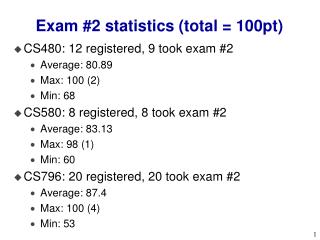
1. Exam #2 statistics (total = 100pt) • CS480: 12 registered, 9 took exam #2 • Average: 80.89 • Max: 100 (2) • Min: 68 • CS580: 8 registered, 8 took exam #2 • Average: 83.13 • Max: 98 (1) • Min: 60 • CS796: 20 registered, 20 took exam #2 • Average: 87.4 • Max: 100 (4) • Min: 53

2. CS480 CS796 CS580

3. PlanningAIMA: 10.1, 10.2, 10.3Follow slides and use textbook as reference

4. Early final exam 12/9/2010?Term paper for CS796 due 12/1/2010

5. “During the Persian Gulf crisis of 1991, U.S. forces deployed a Dynamic Analysis and Replanning Tool, DART (Cross and Walker, 1994), to do automated logistics planning and scheduling for transportation. This involved up to 50,000 vehicles, cargo, and people at a time, and had to account for starting points, destinations, routes, and conflict resolution among all parameters. The AI planning techniques generated in hours a plan that would have taken weeks with older methods. The Defense Advanced Research Project Agency (DARPA) stated that this single application more than paid back DARPA's 30-year investment in Al.”

6. Progression: An action A can be applied to state S iff the preconditions are satisfied in the current state The resulting state S’ is computed as follows: --every variable that occurs in the actions effects gets the value that the action said it should have --every other variable gets the value it had in the state S where the action is applied S’ S Effect Precond STRIPS ASSUMPTION: ONLY variables that have been changed by the action are mentioned in the effect holding(A) ~Clear(A) ~Ontable(A) Ontable(B), Clear(B) ~handempty Pickup(A) Ontable(A) Ontable(B), Clear(A) Clear(B) hand-empty holding(B) ~Clear(B) ~Ontable(B) Ontable(A), Clear(A) ~handempty Pickup(B) Pickup(x) Prec: hand-empty,clear(x),ontable(x) eff: holding(x),~ontable(x),~hand-empty,~Clear(x)

7. A state S can be regressed over an action A (or A is applied in the backward direction to S) Iff: --There is no variable v such that v is given different values by the effects of A and the state S --There is at least one variable v’ such that v’ is given the same value by the effects of A as well as state S The resulting state S’ is computed as follows: -- every variable that occurs in S, and does not occur in the effects of A will be copied over to S’ with its value as in S -- every variable that occurs in the precondition list of A will be copied over to S’ with the value it has in in the precondition list Regression: Termination test: Stop when the state s’ is entailed by the initial state sI Putdown(x) Prec: holding(x) eff: Ontable(x), hand-empty, clear(x), ~holding(x) Stack(x,y) Prec: holding(x), clear(y) eff: on(x,y), ~clear(y), ~holding(x), hand-empty Putdown(A) ~clear(B) holding(A) S’ ~clear(B) hand-empty S Stack(A,B) holding(A) clear(B) Putdown(B)??

8. Progression has higher branching factor Progression searches in the space of complete (and consistent) states Regression has lower branching factor Regression searches in the space of partial states There are 3n partial states (as against 2n complete states) Progression vs. RegressionThe never ending war You can also do bidirectional search stop when a (leaf) state in the progression tree entails a (leaf) state in the regression tree

9. Regression vs. Reversibility • Notice that regression doesn’t require that the actions are reversible in the real world • We only think of actions in the reverse direction during simulation • Normal blocks world is reversible (if you don’t like the effects of stack(A,B), you can do unstack(A,B)). However, if the blocks world has a “bomb” the table action, then normally, there won’t be a way to reverse the effects of that action. • But even with that action we can do regression • For example we can reason that the best way to make table go-away is to add “Bomb” action into the plan as the last action

10. Init: Ontable(A),Ontable(B), Clear(A), Clear(B), hand-empty Goal: ~clear(B), hand-empty Progression vs. Regression • Goal state is partial • if only m of the k state variables are mentioned in a goal specification, then upto 2k-mcomplete state of the world can satisfy our goals! • Sometimes a more complete goal state may provide hints to the agent as to what the plan should be • In the blocks world example, if we also state that On(A,B) as part of the goal (in addition to ~Clear(B)&hand-empty) then it would be quite easy to see what the plan should be. • Initial state is complete • If initial state is partial, then we have “partial observability” (i.e., the agent doesn’t know where it is!) • Because of the asymmetry between init and goal states, progression is in the space of complete states, while regression is in the space of “partial” states. Specifically, for k state variables, there are 2k complete states and 3k “partial” states • (a state variable may be present positively, present negatively or not present at all in the goal specification!)

11. Planning vs. Search: What is the difference? • Search assumes that there is a child-generator and goal-test functions which know how to make sense of the states and generate new states • Planning makes the additional assumption that the states can be represented in terms of state variables and their values • Initial and goal states are specified in terms of assignments over state variables • Which means goal-test doesn’t have to be a blackbox procedure • That the actions modify these state variable values • The preconditions and effects of the actions are in terms of partial assignments over state variables • Given these assumptions certain generic goal-test and child-generator functions can be written • Specifically, we discussed one Child-generator called “Progression”, another called “Regression” • Notice that the additional assumptions made by planning do not change the search algorithms (A*, IDDFS etc)—they only change the child-generator and goal-test functions • In particular, search still happens in terms of search nodes that have parent pointers etc. • The “state” part of the search node will correspond to • “Complete state variable assignments” in the case of progression • “Partial state variable assignments” in the case of regression

12. Relevance, Reachability & Heuristics Reachability: Given a problem [I,G], a (partial) state S is called reachable if there is a sequence [a1,a2,…,ak] of actions, which when executed from state I will lead to a state where S holds Relevance: Given a problem [I,G], a state S is called relevant if there is a sequence [a1,a2,…,ak] of actions, which when executed from state S will lead to a state satisfying G (Relevance is Reachability from goal state) Initial State I S Goal state G S Reachable states Relevant states

13. Relevance, Reachability & Heuristics I G • States that are both reachable and relevant are useful in planning • Progression takes “applicability” of actions into account • Specifically, it guarantees that every state in its search queue is reachable • ..but has no idea whether the states are relevant (constitute progress towards top-level goals) • SO, heuristics for progression need to help it estimate the “relevance” of the states in the search queue • Regression takes “relevance” of actions into account • Specifically, it makes sure that every state in its search queue is relevant • .. But has not idea whether the states in its search queue are reachable • SO, heuristics for regression need to help it estimate the “reachability” of the states in the search queue

14. Subgoal interactions Suppose we have a set of subgoals G1,….Gn Suppose the length of the shortest plan for achieving the subgoals in isolation is l1,….ln We want to know what is the length of the shortest plan for achieving the n subgoals together, l1…n If subgoals are independent: l1..n = l1+l2+…+ln If subgoals have + interactions alone: l1..n < l1+l2+…+ln If subgoals have - interactions alone: l1..n > l1+l2+…+ln If you made “independence” assumption, and added up the individual costs of subgoals, then your resultant heuristic will be perfect if the goals are actually independent inadmissible (over-estimating) if the goals have positive interactions admissible if the goals have negative interactions

15. Scalability came from sophisticated reachability heuristics based on planning graphs.. ..and not from any hand-coded domain-specific control knoweldge Total cost incurred in search Cost of computing the heuristic Cost of searching with the heuristic hC hset-difference h0 h* hP • Not always clear where the total minimum occurs • Old wisdom was that the global min was closer to cheaper heuristics • Current insights are that it may well be far from the cheaper heuristics for many problems • E.g. Pattern databases for 8-puzzle • Plan graph heuristics for planning

16. pqr A2 A1 pq pq A3 A1 pqs A2 p pr A1 psq A3 A3 ps ps A4 pst p q r s p q r s t p A1 A1 A2 A2 A3 A3 A4 Planning Graph and Projection • Envelope of Progression Tree (Relaxed Progression) • Proposition lists: Union of states at kth level • Mutex: Subsets of literals that cannot be part of any legal state • Lowerbound reachability information Planning Graphs can be used as the basis for heuristics! [Blum&Furst, 1995] [ECP, 1997][AI Mag, 2007]

17. Planning Graph Basics pqr A2 A1 pq pq • Envelope of Progression Tree (Relaxed Progression) • Linear vs. Exponential Growth • Reachable states correspond to subsets of proposition lists • BUT not all subsets are states • Can be used for estimating non-reachability • If a state S is not a subset of kth level prop list, then it is definitely not reachable in k steps A3 A1 pqs A2 p pr A1 psq A3 A3 ps ps A4 pst p q r s p q r s t p A1 A1 A2 A2 A3 A3 A4

18. ~Have(cake) eaten(cake) Have(cake) eaten(cake) bake Eat ~Have(cake) eaten(cake) No-op Eat Have(cake) ~eaten(cake) Have(cake) ~eaten(cake) No-op No-op Graph has leveled off, when the prop list has not changed from the previous iteration Have(cake) ~eaten(cake) Don’t look at curved lines for now… The note that the graph has leveled off now since the last two Prop lists are the same (we could actually have stopped at the Previous level since we already have all possible literals by step 2)

19. Blocks world B A Init: Ontable(A),Ontable(B), Clear(A), Clear(B), hand-empty Goal: ~clear(B), hand-empty State variables: Ontable(x) On(x,y) Clear(x) hand-empty holding(x) Initial state: Complete specification of T/F values to state variables --By convention, variables with F values are omitted Goal state: A partial specification of the desired state variable/value combinations --desired values can be both positive and negative Pickup(x) Prec: hand-empty,clear(x),ontable(x) eff: holding(x),~ontable(x),~hand-empty,~Clear(x) Putdown(x) Prec: holding(x) eff: Ontable(x), hand-empty,clear(x),~holding(x) Unstack(x,y) Prec: on(x,y),hand-empty,cl(x) eff: holding(x),~clear(x),clear(y),~hand-empty Stack(x,y) Prec: holding(x), clear(y) eff: on(x,y), ~cl(y), ~holding(x), hand-empty

20. h-A h-B Pick-A Pick-B ~cl-A ~cl-B ~he onT-A onT-A onT-B onT-B cl-A cl-A cl-B cl-B he he

21. h-A on-A-B St-A-B on-B-A h-B Pick-A h-A h-B Pick-B ~cl-A ~cl-A ~cl-B ~cl-B St-B-A ~he ~he onT-A onT-A Ptdn-A onT-A onT-B onT-B onT-B Ptdn-B cl-A cl-A cl-A Pick-A cl-B cl-B cl-B Pick-B he he he

22. Estimating the cost of achieving individual literals (subgoals) Idea: Unfold a data structure called “planning graph” as follows: 1. Start with the initial state. This is called the zeroth level proposition list 2. In the next level, called first level action list, put all the actions whose preconditions are true in the initial state -- Have links between actions and their preconditions 3. In the next level, called first level proposition list, put: Note: A literal appears at most once in a proposition list. 3.1. All the effects of all the actions in the previous level. Links the effects to the respective actions. (If multiple actions give a particular effect, have multiple links to that effect from all those actions) 3.2. All the conditions in the previous proposition list (in this case zeroth proposition list). Put persistence links between the corresponding literals in the previous proposition list and the current proposition list. *4. Repeat steps 2 and 3 until there is no difference between two consecutive proposition lists. At that point the graph is said to have “leveled off” The next 2 slides show this expansion upto two levels

23. Using the planning graph to estimate the cost of single literals: 1. We can say that the cost of a single literal is the index of the first proposition level in which it appears. --If the literal does not appear in any of the levels in the currently expanded planning graph, then the cost of that literal is: -- l+1 if the graph has been expanded to l levels, but has not yet leveled off -- Infinity, if the graph has been expanded (basically, the literal cannot be achieved from the current initial state) Examples: h({~he}) = 1 h ({On(A,B)}) = 2 h({he})= 0 How about sets of literals? see next slide

24. Estimating reachability of sets We can estimate cost of a set of literals in three ways: • Make independence assumption • hsum(p,q,r)= h(p)+h(q)+h(r) • Define the cost of a set of literals in terms of the level where they appear together • h-lev({p,q,r})= The index of the first level of the PG where p,q,r appear together • so, h({~he,h-A}) = 1 • Compute the length of a “relaxed plan” to supporting all the literals in the set S, and use it as the heuristic: hrelax

25. Neither hlev nor hsum work well always P1 P0 A0 True cost of {p1…p100} is 1 (needs just one action reach) Hlev says the cost is 1 Hsum says the cost is 100 Hlev better than Hsum q q B1 p1 B2 p2 B3 p3 p99 B99 p100 B100 P1 P0 A0 q q True cost of {p1…p100} is 100 (needs 100 actions to reach) Hlev says the cost is 1 Hsum says the cost is 100 Hsum better than Hlev p1 p2 B* p3 p99 p100

26. h-sum; h-lev; • H-levis admissible • H-sum in not admissible • H-sum is larger than or equal to H-lev

27. GoalInteractions • To better account for - interactions, we need to start looking into feasibility of subsets of literals actually being true together in a proposition level. • Specifically,in each proposition level, we want to mark not just which individual literals are feasible, • but also which pairs, which triples, which quadruples, and which n-tuples are feasible. (It is quite possible that two literals are independently feasible in level k, but not feasible together in that level) • The idea then is to say that the cost of a set of S literals is the index of the first level of the planning graph, where no subset of S is marked infeasible • The full scale mark-up is very costly, and makes the cost of planning graph construction equal the cost of enumerating the full progression search tree. • Since we only want estimates, it is okay if talk of feasibility of upto k-tuples • For the special case of feasibility of k=2 (2-sized subsets), there are some very efficient marking and propagation procedures. • This is the idea of marking and propagating mutual exclusion relations.

28. Level-off definition? When neither propositions nor mutexes change between levels

29. Mutex Propagation Rules • Two actions a1 and a2 are mutex if any of the following is true: • Inconsistent effects: one action negates the effect of the other. • Interference: one of the effects of one action is the negation of a prediction of the other • Competing needs: one of the predictions of one action is mutually exclusive with a prediction of the other Two propositions P1 and P2 are marked mutexif: allactions supporting P1 are pair-wise mutexwith all actions supporting P2.

30. h-A h-B Pick-A Pick-B ~cl-A ~cl-B ~he onT-A onT-A onT-B onT-B cl-A cl-A cl-B cl-B he he

31. h-A on-A-B St-A-B on-B-A h-B Pick-A h-A h-B Pick-B ~cl-A ~cl-A ~cl-B ~cl-B St-B-A ~he ~he onT-A onT-A Ptdn-A onT-A onT-B onT-B onT-B Ptdn-B cl-A cl-A cl-A Pick-A cl-B cl-B cl-B Pick-B he he he

32. Level-based heuristics on planning graph with mutex relations We now modify the hlev heuristic as follows hlev({p1, …pn})= The index of the first level of the PG where p1, …pn appear together and no pair of them are marked mutex. (If there is no such level, then hlev is set to l+1if the PG is expanded to l levels, and to infinity, if it has been expanded until it leveled off) This heuristic is admissible. With this heuristic, we have a much better handle on both + and - interactions. In our example, this heuristic gives the following reasonable costs: h({~he, cl-A}) = 1 h({~cl-B,he}) = 2 h({he, h-A}) = infinity (because they will be marked mutex even in the final level of the leveled PG) Works very well in practice H({have(cake),eaten(cake)}) = 2

33. How lazy can we be in marking mutexes? • We noticed that hlev is already admissible even without taking negative interactions into account • If we mark mutexes, then hlev can only become more informed • So, being lazy about marking mutexes cannot affect admissibility • However, being over-eager about marking mutexes (i.e., marking non-mutex actions mutex) does lead to loss of admissibility

34. Some observations about the structure of the PG 1. If an action a is present in level l, it will be present in all subsequent levels. 2. If a literal p is present in level l, it will be present in all subsequent levels. 3. If two literals p,q are not mutex in level l, they will never be mutex in subsequent levels --Mutex relations relax monotonically as we grow PG

35. Summary • Planning and search • Progression • Regression • Planning graph and heuristics • Goal interactions and mutual exclusion