Bioinformatics 3 V 5 – Robustness and Modularity
420 likes | 585 Vues
Bioinformatics 3 V 5 – Robustness and Modularity. Mon, Nov 4, 2013. Network Robustness. Network = set of connections. Failure events:. • loss of edges • loss of nodes (together with their edges). → loss of connectivity • paths become longer (detours required)

Bioinformatics 3 V 5 – Robustness and Modularity
E N D
Presentation Transcript
Bioinformatics 3V 5 – Robustness and Modularity Mon, Nov 4, 2013
Network Robustness Network = set of connections Failure events: • loss of edges • loss of nodes (together with their edges) → loss of connectivity • paths become longer (detours required) • connected components break apart → network characteristics change →Robustness = how much does the network (not) change when edges/nodes are removed
Random vs. Scale-Free 130 nodes, 215 edges The top 5 nodes with the highest kconnect to… … 27% of the network … 60% of the network Albert, Jeong, Barabási, Nature406 (2000) 378
network diameter fraction of nodes removed Failure vs. Attack Failure: remove randomly selected nodes Attack: remove nodes with highest degrees SF: scale-free network -> attack E: exponential (random) network -> failure / attack SF: failure N = 10000, L = 20000, but effect is size-independent; SF network diameter increases strongly when network is attacked but not when nodes fail randomly Albert, Jeong, Barabási, Nature406 (2000) 378
network diameter fraction of nodes removed Two VINs Scale-free: • very stable against random failure ("packet re-rooting") • very vulnerable against dedicated attacks ("9/11") http://moat.nlanr.net/Routing/rawdata/ : 6209 nodes and 12200 links (2000) WWW-sample containing 325729 nodes and 1498353 links Albert, Jeong, Barabási, Nature406 (2000) 378
cluster sizes S and <s> fraction of nodes removed Network Fragmentation Relative size of the largest clusters S Average size of the isolated clusters <s> (except the largest one) Random network: • no difference between attack and failure (homogeneity) • fragmentation threshold at fc ≳ 0.28 (S ≈ 0) Scale-free network: • delayed fragmentation and isolated nodes for failure • critical breakdown under attack at fc ≈ 0.18 Albert, Jeong, Barabási, Nature406 (2000) 378
Mesoscale properties of networks- identify cliques and highly connected clusters Most relevant processes in biological networks correspond to the mesoscale (5-25 genes or proteins) not to the entire network. However, it is computationally enormously expensive to study mesoscale properties of biological networks. e.g. a network of 1000 nodes contains 1 1023 possible 10-node sets. Spirin & Mirny analyzed combined network of protein interactions with data from CELLZOME, MIPS, BIND: 6500 interactions.
Identify connected subgraphs The network of protein interactions is typically presented as an undirected graph with proteins as nodes and protein interactions as undirected edges. Aim: identify highly connected subgraphs (clusters) that have more interactions within themselves and fewer with the rest of the graph. A fully connected subgraph, or clique, that is not a part of any other clique is an example of such a cluster. The „maximum clique problem“ – finding the largest clique in a given graph is known be NP-hard. In general, clusters need not to be fully connected. Measure density of connections by where n is the number of proteins in the cluster and m is the number of interactions between them. Spirin, Mirny, PNAS 100, 12123 (2003) 9
Clique and Maximal Clique A clique is a fully connected sub-graph, that is, a set of nodes that are all neighbors of each other. In this example, the whole graph is a clique and consequently any subset of it is also a clique, for example {a,c,d,e} or {b,e}. A maximal clique is a clique that is not contained in any larger clique. Here only {a,b,c,d,e} is a maximal clique. Gagneur et al. Genome Biology 5, R57 (2004)
(method I) Identify all fully connected subgraphs (cliques) The general problem - finding all cliques of a graph - is very hard. Because the protein interaction graph is sofar very sparse (the number of interactions (edges) is similar to the number of proteins (nodes), this can be done quickly. To find cliques of size n one needs to enumerate only the cliques of size n-1. The search for cliques starts with n = 4, pick all (known) pairs of edges (6500 6500 protein interactions) successively. For every pair A-B and C-D check whether there are edges between A and C, A and D, B and C, and B and D. If these edges are present, ABCD is a clique. For every clique identified, ABCD, pick all known proteins successively. For every picked protein E, if all of the interactions E-A, E-B, E-C, and E-D exist, then ABCDE is a clique with size 5. Continue for n = 6, 7, ... The largest clique found in the protein-interaction network has size 14. Spirin, Mirny, PNAS 100, 12123 (2003)
(I) Identify all fully connected subgraphs (cliques) These results include, however, many redundant cliques. For example, the clique with size 14 contains 14 cliques with size 13. To find all nonredundant subgraphs, mark all proteins comprising the clique of size 14, and out of all subgraphs of size 13 pick those that have at least one protein other than marked. After all redundant cliques of size 13 are removed, proceed to remove redundant twelves etc. In total, only 41 nonredundant cliques with sizes 4 - 14 were found by Spirin & Mirny. Spirin, Mirny, PNAS 100, 12123 (2003)
Statistical significance of cliques Number of complete cliques (Q = 1) as a function of clique size enumerated in the network of protein interactions (red) and in randomly rewired graphs (blue, averaged >1,000 graphs where number of interactions for each protein is preserved). Inset shows the same plot in log-normal scale. Note the dramatic enrichment in the number of cliques in the protein-interaction graph compared with the random graphs. Most of these cliques are parts of bigger complexes and modules. Spirin, Mirny, PNAS 100, 12123 (2003)
(method II) Monte Carlo Simulation Use MC to find a tight subgraph of a predetermined number of M nodes. At time t = 0, a random set of M nodes is selected. For each pair of nodes i,j from this set, the shortest path Lijbetween i and j on the graph is calculated. Define L0 := sum of all shortest paths Lijfrom this set. At every time step one of the M nodes is picked at random, and one node is picked at random out of all its neighbors. Calculate the new sum of all shortest paths, L1, if the original node were to be replaced by this neighbor. If L1 < L0, accept replacement with probability 1. If L1 > L0, accept replacement with probability where T is the effective temperature. Spirin, Mirny, PNAS 100, 12123 (2003)
(method II) Monte Carlo Simulation Every tenth time step an attempt is made to replace one of the nodes from the current set with a node that has no edges to the current set to avoid getting caught in an isolated disconnected subgraph. This process is repeated (i) until the original set converges to a complete subgraph, or (ii) for a predetermined number of steps, after which the tightest subgraph (the subgraph corresponding to the smallest L0) is recorded. The recorded clusters are merged and redundant clusters are removed. Spirin, Mirny, PNAS 100, 12123 (2003)
Merging Overlapping Clusters A simple statistical test shows that nodes which have only one link to a cluster are statistically insignificant. Clean such statistically insignificant members first. Then merge overlapping clusters: For every cluster Aifind all clusters Akthat overlap with this cluster by at least one protein. For every such found cluster calculate Q value of a possible merged cluster AiU Ak . Record cluster Abest(i) which gives the highest Q value if merged with Ai. After the best match is found for every cluster, every cluster Ai is replaced by a merged cluster AiU Abest(i) unless AiU Abest(i) is below a certain threshold value for QC. This process continues until there are no more overlapping clusters or until merging any of the remaining clusters will make a cluster with Q value lower than QC. Spirin, Mirny, PNAS 100, 12123 (2003)
Statistical significance of complexes and modules Distribution of Q of clusters found by the MC search method. Red bars: original network of protein interactions. Blue curves: randomly rewired graphs. -> Clusters in the protein network have many more interactions than their counterparts in the random graphs. Spirin, Mirny, PNAS 100, 12123 (2003)
Architecture of protein network Fragment of the protein network. Nodes and interactions in discovered clusters are shown in bold. Nodes are colored by functional categories in MIPS: red, transcription regulation; blue, cell-cycle/cell-fate control; green, RNA processing; and yellow, protein transport. Complexes shown are the SAGA/TFIID complex (red), the anaphase-promoting complex (blue), and the TRAPP complex (yellow). Spirin, Mirny, PNAS 100, 12123 (2003)
Discovered functional modules • Examplesofdiscoveredfunctionalmodules. • A moduleinvolved in cell-cycleregulation. This moduleconsistsofcyclins (CLB1-4 and CLN2) andcyclin-dependentkinases (CKS1 and CDC28) and a nuclearimportprotein (NIP29). Althoughtheyhavemanyinteractions, theseproteinsare not present in thecellatthe same time. • (B) Pheromone signaltransductionpathway in thenetworkofprotein–proteininteractions. This moduleincludesseveral MAPK (mitogen-activatedproteinkinase) and MAPKK (mitogen-activatedproteinkinasekinase) kinases, aswellasotherproteinsinvolved in signaltransduction. These proteins do not form a singlecomplex; rather, theyinteract in a specificorder. Spirin, Mirny, PNAS 100, 12123 (2003)
Analysis of identified complexes Comparison of discovered complexes and modules with complexes derived experimentally (BIND and Cellzome) and complexes catalogued in MIPS. Discovered complexes are sorted by the overlap with the best-matching experimental complex. The overlap is defined as the number of common proteins divided by the number of proteins in the best-matching experimental complex. -> The first 31 complexes match exactly, and another 11 have overlap above 65%. Inset shows the overlap as a function of the size of the discovered complex. Note that discovered complexes of all sizes match very well with known experimental complexes. Discovered complexes that do not match with experimental ones constitute our predictions. Spirin, Mirny, PNAS 100, 12123 (2003)
Robustness of clusters found Model effect of false positives in experimental data: randomly reconnect, remove or add 10-50% of interactions in network. Recovery probability plotted as a function of the fraction of altered links. Black: links are rewired. Red, links are removed; Green, links are added. Circles: probability to recover 75% of the original cluster; Triangles: probability to recover 50%. Noise in the form of removal or additions of links has less deteriorating effect than random rewiring. About 75% of clusters can still be found when 10% of links are rewired. Spirin, Mirny, PNAS 100, 12123 (2003)
Summary Analysis of meso-scale properties demonstrated the presence of highly connected clusters of proteins in a network of protein interactions -> strongly supports suggested modular architecture of biological networks. There exist 2 types of clusters: protein complexes and dynamic functional modules. Both have more interactions among their members than with the rest of the network. Dynamic modules cannot be purified in experiments because they are not assembled as a complex at any single point in time. Computational analysis allows detection of such modules by integrating pairwise molecular interactions that occur at different times and places. However, computational analysis alone does not allow to distinguish between complexes and modules or between transient and simultaneous interactions.
Reducing Network Complexity? Is there a representation that highlights the structure of these networks??? • Modular Decomposition (Gagneur, …, Casari, 2004) • Network Compression (Royer, …, Schröder, 2008)
Shared Components Shared components = proteins or groups of proteins occurring in different complexes are fairly common. A shared component may be a small part of many complexes, acting as a unit that is constantly reused for its function. Also, it may be the main part of the complex e.g. in a family of variant complexes that differ from each other by distinct proteins that provide functional specificity. Aim: identify and properly represent the modularity of protein-protein interaction networks by identifying the shared components and the way they are arranged to generate complexes. Gagneur et al. Genome Biology 5, R57 (2004) Georg Casari, Cellzome (Heidelberg)
Modular Decomposition of a Graph Module := set of nodes that have the same neighbors outside of the module trivial modules: {a}, {b}, …, {g} {a, b, …, g} non-trivial modules: {a, b}, {a, c}, {b, c} {a, b, c} {e, f} Quotient: representative node for a module Iterated quotients → labeled tree representing the original network → "modular decomposition" Gagneur et al, Genome Biology5 (2004) R57
Quotients Series: all included nodes are direct neighbors (= clique) → Parallel: all included nodes are non-neighbors → Prime: "anything else" (best labeled with the actual structure) →
A Simple Recursive Example parallel series prime Gagneur et al, Genome Biology5 (2004) R57
Results from protein complex purifications (PCP), e.g. TAP Different types of data: • Y2H: detects direct physical interactions between proteins • PCP by tandem affinity purification with mass-spectrometric identification of the protein components identifies multi-protein complexes → Molecular decomposition will have a different meaning due to different semantics of such graphs. Here, we focus analysis on PCP content. PCP experiment: select bait protein where TAP-label is attached → Co-purify protein with those proteins that co-occur in at least one complex with the bait protein. Gagneur et al. Genome Biology 5, R57 (2004)
Data from Protein Complex Purification Graphs and module labels from systematic PCP experiments: (a) Two neighbors in the network are proteins occurring in a same complex. (b) Several potential sets of complexes can be the origin of the same observed network. Restricting interpretation to the simplest model (top right), the series module reads as a logical AND between its members. (c) A module labeled ´parallel´ corresponds to proteins or modules working as strict alternatives with respect to their common neighbors. (d) The ´prime´ case is a structure where none of the two previous cases occurs. Gagneur et al. Genome Biology 5, R57 (2004)
Real World Examples Two examples of modular decompositions of protein-protein interaction networks. In each case from top to bottom: schemata of the complexes, the corresponding protein-protein interaction network as determined from PCP experiments, and its modular decomposition (MOD). (a) Protein phosphatase 2A. Parallel modules group proteins that do not interact but are functionally equivalent. Here these are the catalytic proteins Pph21 and Pph22 (module 2) and the regulatory proteins Cdc55 and Rts1 (module 3), connected by the Tpd3 „backbone“. Notes: • Graph does not show functional alternatives!!! • other decompositions also possible Gagneur et al. Genome Biology 5, R57 (2004)
RNA polymerases I, II and III Again: modular decompositon easier to comprehend than graph Gagneur et al. Genome Biology 5, R57 (2004)
Summary Modular decomposition of graphs is a well-defined concept. • One can proof thoroughly for which graphs a modular decomposition exists. • Efficient O(m + n) algorithms exist to compute the decomposition. However, experiments have shown that biological complexes are not strictly disjoint. They often share components → separate complexes do not always fulfill the strict requirements of modular graph decomposition. Also, there exists a „danger“ of false-positive or false-negative interactions. →other methods, e.g., for detecting communities (Girven & Newman) or clusters (Spirin & Mirny) are more suitable for identification of complexes because they are more sensitive.
Power Graph Analysis PLoS Comp Biol4 (2008) e1000108 Lossless compact abstract representation of graphs: • Power nodes = set of nodes (criterion for grouping?) • Power edges = edges between power nodes Exploit observation that cliques and bi-cliques are abundant in real networks →explicitly represented in power graphs
Power Nodes In words: "… if two power nodes are connected by a power edge in G', this means in G that allnodes of the first power node are connected to all nodes of the second power node. Similarly, if a power node is connected to itself by a power edge in G', this means that all nodes in the power node are connected to each other by edges in G. With: "real-world" graph G = {V, E} power graph G' = {V', E'} Royer et al, PLoS Comp Biol4 (2008) e1000108
Power Graph Analysis Algorithm Two conditions: • power node hierarchy condition: two power nodes are either disjoint, or one is included in the other one • power edge disjointness condition: each edge of the original graph is represented by one and only one power edge Algorithm: 1) identify potential power nodes with hierarchical clustering based on neighborhood similarity 2) greedy power edge search Royer et al, PLoS Comp Biol4 (2008) e1000108
Complex = Star or Clique? In pull-down experiments: Bait is used to capture complexes of prey proteins → do they all just stick to the bait or to each other? spoke model →underestimates connectivity matrix model →overestimates connectivity Royer et al, PLoS Comp Biol4 (2008) e1000108
Casein Kinase II Complex → Power graph: compressed and cleaner representation Royer et al, PLoS Comp Biol4 (2008) e1000108
Various Similarities Royer et al, PLoS Comp Biol4 (2008) e1000108
Network Compression Power graph analysis: group nodes with similar neighborhood → often functionally related proteins end up in one power node Lossless compression of graphs: 38…85% edge reduction for biological networks Royer et al, PLoS Comp Biol4 (2008) e1000108
Some PPI Networks For some time: "Biological networks are scale-free…" Y2H PPI network from Uetz etal, Nature403 (2003) 623 P(k) compared to a power law However, there are some doubts… → next lecture
Summary What you learned today: • Network robustness scale-free networks are failure-tolerant, but fragile to attacks <=> the few hubs are important => immunize hubs! • Modules in networks => modular decomposition => power graph analysis Next lecture: • Are biological networks scale-free? (other models?) • Network growth mechanisms Short Test #1: Mon, Nov. 11 (covers lectures V2-V6)