Download
1 / 54
540 likes | 674 Vues
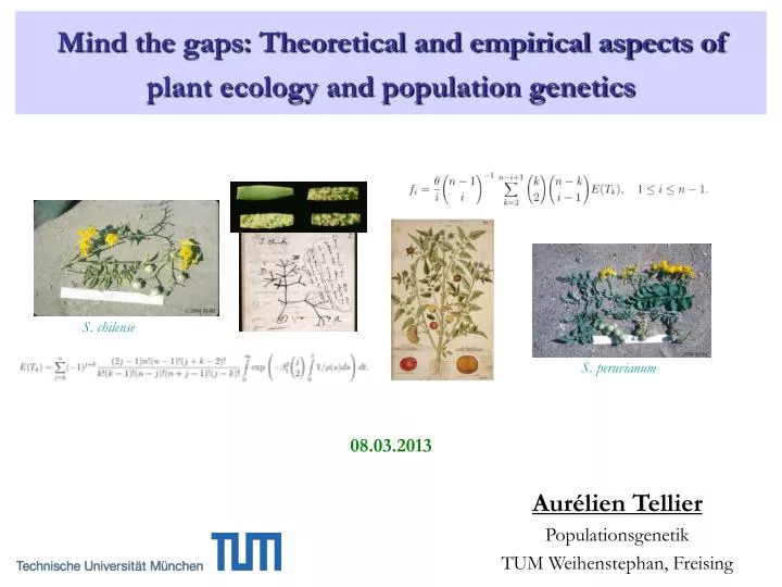
S. chilense. S. peruvianum. Mind the gaps: Theoretical and empirical aspects of plant ecology and population genetics. 08.03.2013. Aurélien Tellier Populationsgenetik TUM Weihenstephan, Freising. Research interests: Ecology and genetics/genomics. How do plants adapt to their environment?

E N D
S. chilense S. peruvianum Mind the gaps: Theoretical and empirical aspects of plant ecology and population genetics 08.03.2013 Aurélien Tellier Populationsgenetik TUM Weihenstephan, Freising
Research interests:Ecology and genetics/genomics How do plants adapt to their environment? Major aims • Determining the genetic processes involved in adaptation • How genetic variation is shaped by evolutionary/ecological processes Ecology ecological time scale Influence of environmentObservable variation in phenotypes Genomics evolutionary time scale Apparition and fixation of mutationsRandom processes (drift, migration)
2011 Research interests: Two systems Plant-parasite coevolution Seed banks and seed dormancy
Population genetics: 4 evolutionary forces random genomic processes(mutation, duplication, recombination, gene conversion) molecular diversity natural selection random spatialprocess (migration) random demographicprocess (drift) • Investigate the laws governing the genetic structure of populations R.A. Fisher, S. Wright, J.B.S. Haldane, …, M. Kimura, T. Ohta, …, B. Charlesworth, J. Maynard-Smith • Coalescent theory is a tool to infer past evolution from sequence data
Overview of the immune system in plants unspecific immunity specific immunity pathogen pathogen plant cell direct recognition indirect recognition effectors modification plant cell ‘guardee’ (pathogen target) R proteins ‘guard’ signalling signalling basal defense response specific defense response (HR)
The Gene-For-Gene relationship Plant Susceptible Resistant Fungus Avirulent Virulent
Natural selection in coevolution (1) Virulence increases pathogen fitness on resistant plants Resistance increases plant fitness in present of pathogen Brown and Tellier, Annual Review Phytopathology, 2011
Natural selection in coevolution (2) Cost of resistance to plant fitness Cost of virulence to pathogen fitness Brown and Tellier, Annual Review Phytopathology, 2011
Equilibrium points : instability Freq. of virulence Unstable equilibrium 1 0 1 0 Stable equilibria Frequency of resistance
Equilibrium points : instability Freq. of virulence Stable equilibria 1 Unstable equilibrium 0 1 0 Frequency of resistance
Equilibrium points : stability Freq. of virulence Stable equilibrium 1 0 1 0 Frequency of resistance
Equilibrium points : stability Freq. of virulence Stable equilibrium 1 0 1 0 Frequency of resistance
( ) R ′ R (1−u)(1−s+sA) . = r r 1−s Why the simple model is unstable (1) s = cost of disease u = cost of resistance Taking log of ratio, ρ = log(R/r) … maths easier! log ρ′ − log ρ = Δρ log ρ′ − log ρ= log(1−u) + log(1−s−sA) − log(1−s) The change in R depends on Abut not on R itself
( ) A ′ A 1−cR . = a a 1−b Why the simple model is unstable (1) c = cost of AVR on RES plant b = cost of virulence Taking log of ratio, α = log(A/a) log α′ − log α = Δα log ρ′ − log ρ= log(1−cR) − log(1−b) The change in A depends on Rbut not on A itself Hence dΔρ/dR + dΔα/dA= 0 and stability is impossible
(-1,0) Requirements for stable polymorphism Jacobian Matrix • The eigenvalues 1,2 = iof the Jacobian Matrix should be in a circle centered on (-1,0) in the complex plane <0the sum of the diagonal coefficients of the Jacobian matrix - Tellier and Brown, Proc. Roy. Soc. B, 2007
Requirements for stable polymorphism • Avirulence selects for increased resistance • Resistance selects for increased virulence = indirect frequency-dependent selection → graph of alleles frequencies (R,a) spirals • Selection for RES weaker as RES more common • Or selection for avr weaker as avr more common = direct frequency-dependent selection → graph spirals to a stable equilibrium point Tellier and Brown, Proc. Roy. Soc. B, 2007
Boom andBustcycle: stableandunstabledynamics Brown and Tellier Ann Rev Phytopat 2011 • Factors promoting stable dynamics: • Biological factors (life history traits): • Polycylicity = several pathogen generations/host generation (Tellier and Brown, Proc Roy Soc B, 2007) • Perenniality or seed banks in host (Tellier and Brown, Am Nat, 2009) • Genetic factors:Epistasis among R-genes and virulence genes (Tellier and Brown, Genetics, 2007) • Ecological factors:Environmental variability in space (Laine and TellierOikos 2008; Tellier and Brown BMC EvolBiol 2011)
Stableandunstabledynamics Brown and Tellier Ann Rev Phytopat 2011 Biological factors (life history traits):Polycylicity, perenniality or seed banks Genetic factors:Epistasis Ecological factors:Environmental variability in space (see work by Laine, Thrall, Burdon,…) Expect to find often stable dynamics in natural populations! (and conversely more unstable dynamics in agro-systems)
Whyisitimportanttoknowthestability/unstability? Brown and Tellier Ann Rev Phytopat 2011 balancing selection (trench warfare) ndFDS selection model positive selection (arms race) selective sweeps model host pathogen Stahl et al. Nature 1999, Holub Nat Rev Genet 2001, Woolhouse et al. Nat Rev Genet 2002
„Naive“ Predictions on genomicsignatures Ebert Curr Opin Microbiol 2008 selective sweeps ndFDS selection model host pathogen
Predictions on genomic signatures selective sweeps ndFDS selection model host pathogen Sample n = 8 One type present(AVR or avr RES or res) avr / res AVR / RES • Short tree => low genetic diversity • Star like genealogy => excess of singleton SNPs • Negative value of Tajima’s D (<0) • Long tree => high genetic diversity • Long internal branches => excess of intermediate frequency SNPs • Positive value of Tajima’s D (>0)
Genomicsignatureofbalancingselection Neutral mutations segregating next to the selected SNPno intra-locus recombination(Charlesworth et al. Genet Res 1997 ) AVR or RES avr or res neutral SNPs Causal SNP
Genomicsignatureofselectivesweeps Neutral mutations segregating next to the selected SNPno intra-locus recombination(Maynard-Smith and Haig Genet Res 1974) RES neutral SNPs Causal SNP
Genome scansto find genes undercoevolution selective sweeps ndFDS selection model host pathogen Based on statistics of genealogies: Tajima’s D, haplotypes…
However, few genes showthesetypicalsignatures… Ex: RPM1 in Arabidopsis thaliana(Stahl et al. Nature 1999, Bergelson et al. Science 2001)Ptoin Solanum Peruvianum (Rose et al. Genetics 2007) Cao et al. Nat Genet 2011; Guo et al. Plant Physiol 2011 Bakker et al. Plant Cell 2006; Bakker et al. Genetics 2008
Why so littlegenomicevidenceforcoevolution? A major draw back of current theory is that it is based on deterministic models and short-term ecological models Questions: 1) What is the role of genetic drift for stability or allele fixation? 2) In finite populations, can stable dynamics lead to fixation of alleles? Under which conditions? 3) Are dynamics in the arms race model slower than in the trench warfare model? 4) Expectations for genomic signatures under GFG models? Exemple of a stable model in finite population (N = 3000)
Finite size model How? We build a model of host and parasite with finite size with genetic drift (NH = NP) + mutation between AVR ↔ avr and RES ↔ res Assess population genetics statistics: time to fixation; how often are alleles close to fixation (freq<0.05 or freq>0.95); number of cycles and amplitude, periods of cycles For 10,000 generations and various parameter combinations
UNSTABLE dynamics 1) What is the role of genetic drift for stability or allele fixation? Number of coevolutionary cycles Fast cycling Slow cycling Increasing mutational input (Nμ) Fixed mutation rate μ = 10-5
UNSTABLE dynamics 1) What is the role of genetic drift for stability or allele fixation? Number of coevolutionary cycles Fast cycling Slow cycling Fixed population mutation rate θ= 4Nμ = 0.01 Result 1: genetic drift has small effect on speed of coevolutionary cycles Mutational input determines the speed of cycles
UNSTABLE dynamics 1) What is the role of genetic drift for stability or allele fixation? Percentage of time that allele RES is fixed or near fixation Often fixed Never fixed Fixed population mutation rate θ = 4Nμ = 0.01 Result 2: Drift affects the time of allele fixationResistance can only be fixed in plant populations of small size
STABLE dynamics 2) In finite populations, can stable dynamics lead to fixation of alleles? What conditions? Percentage of time of susceptible allele res fixed or near fixation Often fixed= sweeps Never fixed = polymorphism Fixed population mutation rate θ = 4Nμ = 0.01 Result 3:Genetic drift alone is responsible for driving stable cycles to fixationMore pronounced for small population sizes
STABLE dynamics 2) What conditions for fixation of alleles in stable model? Result 4: The location of the equilibrium point determines the fixation probability (=> importance of costs) BUT amplitude and period of cycles affect weakly fixation and speed of coevolution
STABLE vs UNSTABLE dynamics 3) Are dynamics in the arms race model slower than in the trench warfare model? Number of coevolutionary cycles Unstable model = selective sweeps Stable model = balancing selection Fast cycling Slow cycling Result 5: For low values of costs, the speed of coevolution is similar between dynamics (in contradiction to Woolhouse et al., Ebert)
Expected genomic signatures of coevolution 4) Expectations for genomic signatures of GFG models? How?Simulate frequency dynamics + coalescent theory (Kingman TPB 1982, Donnelly, Tavare, Nordborg, Barton, Etheridge,…) to simulate genetic data Sample = 40 plants and 40 parasites ..A……….T………T……………..G…… ..T……….T………G……………..C…… ..A……….A………G……………..C…… Past = start of selection Present = sample
Expected genomic signatures of coevolution 4) Expectations for genomic signatures under GFG models? Tajima’s D for Unstable and Stable dynamics over range of parametersMean of Tajima’s D over 2,000 replicates, N=1,000 and =10-4 Balancing selection Cost of being diseased (s) 0.0 0.1 0.2 0.3 0.4 0.5 0.6 0.00 0.05 0.10 0.15 0.20 0.25 0.30 0.00 0.05 0.10 0.15 0.20 0.25 0.30 Selective sweeps cost of virulence = cost of resistance (u=b)
Expected genomic signatures of coevolution 4) Expectations for genomic signatures under GFG models? Tajima’s D for Unstable and Stable dynamics over range of parametersMean of Tajima’s D over 2,000 replicates, N=1,000 and =10-4 Balancing selection Cost of being diseased (s) 0.0 0.1 0.2 0.3 0.4 0.5 0.6 0.00 0.05 0.10 0.15 0.20 0.25 0.30 0.00 0.05 0.10 0.15 0.20 0.25 0.30 Selective sweeps cost of virulence = cost of resistance (u=b) Result 8: Balancing selection signature is not observable in populations with small N
Expected genomic signatures of coevolution 4) Expectations for genomic signatures under GFG models? Tajima’s D for Unstable and Stable dynamics over range of parametersMean of Tajima’s D over 2,000 replicates, N=10,000 and =10-5 Balancing selection Cost of being diseased (s) 0.0 0.1 0.2 0.3 0.4 0.5 0.6 0.00 0.05 0.10 0.15 0.20 0.25 0.30 0.00 0.05 0.10 0.15 0.20 0.25 0.30 Selective sweeps cost of virulence = cost of resistance (u=b)
Expected genomic signatures of coevolution 4) Expectations for genomic signatures under GFG models? Tajima’s D for Unstable and Stable dynamics over range of parametersMean of Tajima’s D over 2,000 replicates, N=10,000 and =10-5 Balancing selection Cost of being diseased (s) 0.0 0.1 0.2 0.3 0.4 0.5 0.6 0.00 0.05 0.10 0.15 0.20 0.25 0.30 0.00 0.05 0.10 0.15 0.20 0.25 0.30 Selective sweeps cost of virulence = cost of resistance (u=b) Result 8: Balancing selection signature is only observable in populations with high N and in parasites
Expected genomic signatures of coevolution 4) Expectations for genomic signatures under GFG models? Tajima’s D for Unstable and Stable dynamics over range of parametersMean of Tajima’s D over 2,000 replicates, N=1,000 and =10-5 Balancing selection Cost of being diseased (s) 0.0 0.1 0.2 0.3 0.4 0.5 0.6 0.00 0.05 0.10 0.15 0.20 0.25 0.30 0.00 0.05 0.10 0.15 0.20 0.25 0.30 Selective sweeps cost of virulence = cost of resistance (u=b)
Expected genomic signatures of coevolution 4) Expectations for genomic signatures under GFG models? Tajima’s D for Unstable and Stable dynamics over range of parametersMean of Tajima’s D over 2,000 replicates, N=1,000 and =10-5 Balancing selection Cost of being diseased (s) 0.0 0.1 0.2 0.3 0.4 0.5 0.6 0.00 0.05 0.10 0.15 0.20 0.25 0.30 0.00 0.05 0.10 0.15 0.20 0.25 0.30 Selective sweeps cost of virulence = cost of resistance (u=b) Result 8: Balancing selection signature is not observable in populations with small N
Expected genomic signatures of coevolution 4) Expectations for genomic signatures under GFG models? Tajima’s D for Unstable and Stable dynamics over range of parametersMean of Tajima’s D over 2,000 replicates, N=10,000 and =10-6 Balancing selection Cost of being diseased (s) 0.0 0.1 0.2 0.3 0.4 0.5 0.6 0.00 0.05 0.10 0.15 0.20 0.25 0.30 0.00 0.05 0.10 0.15 0.20 0.25 0.30 Selective sweeps cost of virulence = cost of resistance (u=b)
Expected genomic signatures of coevolution 4) Expectations for genomic signatures under GFG models? Tajima’s D for Unstable and Stable dynamics over range of parametersMean of Tajima’s D over 2,000 replicates, N=10,000 and =10-6 Balancing selection Cost of being diseased (s) 0.0 0.1 0.2 0.3 0.4 0.5 0.6 0.00 0.05 0.10 0.15 0.20 0.25 0.30 0.00 0.05 0.10 0.15 0.20 0.25 0.30 Selective sweeps cost of virulence = cost of resistance (u=b) Result 8: Balancing selection signature is only observable in populations with high N and in parasites
Expected genomic signatures of coevolution Tajima’s D for Unstable and Stable dynamics over range of parametersover 2,000 replicates, N=1,000 and =10-4 Mean Mode Balancing selection Cost of being diseased (s) 0.0 0.1 0.2 0.3 0.4 0.5 0.6 0.00 0.05 0.10 0.15 0.20 0.25 0.30 0.00 0.05 0.10 0.15 0.20 0.25 0.30 Selective sweeps cost of virulence = cost of resistance (u=b)
Expected genomic signatures of coevolution Tajima’s D for Unstable and Stable dynamics over range of parametersover 2,000 replicates, N=1,000 and =10-4 Mean Mode Balancing selection Cost of being diseased (s) 0.0 0.1 0.2 0.3 0.4 0.5 0.6 0.00 0.05 0.10 0.15 0.20 0.25 0.30 0.00 0.05 0.10 0.15 0.20 0.25 0.30 Selective sweeps cost of virulence = cost of resistance (u=b)
Expected genomic signatures of coevolution Tajima’s D for Unstable and Stable dynamics over range of parametersover 2,000 replicates, N=10,000 and =10-5 Mean Mode Balancing selection Cost of being diseased (s) 0.0 0.1 0.2 0.3 0.4 0.5 0.6 0.00 0.05 0.10 0.15 0.20 0.25 0.30 0.00 0.05 0.10 0.15 0.20 0.25 0.30 Selective sweeps cost of virulence = cost of resistance (u=b)
Expected genomic signatures of coevolution Tajima’s D for Unstable and Stable dynamics over range of parametersover 2,000 replicates, N=10,000 and =10-5 Mean Mode Balancing selection Cost of being diseased (s) 0.0 0.1 0.2 0.3 0.4 0.5 0.6 0.00 0.05 0.10 0.15 0.20 0.25 0.30 0.00 0.05 0.10 0.15 0.20 0.25 0.30 Selective sweeps cost of virulence = cost of resistance (u=b)
Expected genomic signatures of coevolution Tajima’s D for Unstable and Stable dynamics over range of parametersover 2,000 replicates, N=10,000 and =10-6 Mean Mode Balancing selection Cost of being diseased (s) 0.0 0.1 0.2 0.3 0.4 0.5 0.6 0.00 0.05 0.10 0.15 0.20 0.25 0.30 0.00 0.05 0.10 0.15 0.20 0.25 0.30 Selective sweeps cost of virulence = cost of resistance (u=b)
Expected genomic signatures of coevolution Tajima’s D for Unstable and Stable dynamics over range of parametersover 2,000 replicates, N=10,000 and =10-6 Mean Mode Balancing selection Cost of being diseased (s) 0.0 0.1 0.2 0.3 0.4 0.5 0.6 0.00 0.05 0.10 0.15 0.20 0.25 0.30 0.00 0.05 0.10 0.15 0.20 0.25 0.30 Selective sweeps cost of virulence = cost of resistance (u=b)
Conclusions • 1) What is the role of genetic drift for stability or allele fixation? • 2) In finite populations, can stable dynamics lead to fixation of alleles? Under which conditions? • Genetic drift does not influence the speed of coevolution, but the fixation rate of alleles • Alleles can get fixed in a stable model (contrary to common wisdom) • Resistance alleles only get fixed in small populations!!! Diversifying selection at Rgenes must have occurred in small plant populations • 3) Are dynamics in the arms race model slower than in the trench warfare model? • No, for most parameter values there is no difference between the speed of coevolution • Relevance for field studies following changes in allele frequencies • 4) Expectations for genomic signatures under GFG models? • Unstable dynamics can lead to a big variation in genomic signatures • Bad news:almost no chance to find balancing selection in genome scans in plants (ex. Arabidopsis thaliana), AND costs determine the equilibrium point • Good news: genome scans can be used to find balancing selection in parasites
James Brown Thomas Städler Thanks to hazards of migration Wolfgang Stephan Stefan Laurent Daniel Živković Mamadou Mboup Katharina Böndel Anja Hörger T. Giraud (University Paris 13) J. Enjalbert (INRA, France) A.L. Laine (University Helsinki)