Download
1 / 78
780 likes | 954 Vues
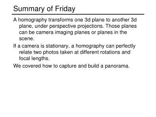
Summary of Friday. A homography transforms one 3d plane to another 3d plane, under perspective projections. Those planes can be camera imaging planes or planes in the scene.

E N D
Summary of Friday • A homography transforms one 3d plane to another 3d plane, under perspective projections. Those planes can be camera imaging planes or planes in the scene. • If a camera is stationary, a homography can perfectly relate two photos taken at different rotations and focal lengths. • We covered how to capture and build a panorama.
Automatic Image Alignment © Mike Nese cs195g: Computational Photography James Hays, Brown, Spring 2010 Slides from Alexei Efros, Steve Seitz, and Rick Szeliski
Live Homography DEMO • Check out panoramio.com “Look Around” feature! Also see OpenPhoto VR: http://openphotovr.org/
Image Alignment • How do we align two images automatically? • Two broad approaches: • Feature-based alignment • Find a few matching features in both images • compute alignment • Direct (pixel-based) alignment • Search for alignment where most pixels agree
Direct Alignment • The simplest approach is a brute force search (hw1) • Need to define image matching function • SSD, Normalized Correlation, edge matching, etc. • Search over all parameters within a reasonable range: • e.g. for translation: • for tx=x0:step:x1, • for ty=y0:step:y1, • compare image1(x,y) to image2(x+tx,y+ty) • end; • end; • Need to pick correct x0,x1 and step • What happens if step is too large?
Direct Alignment (brute force) • What if we want to search for more complicated transformation, e.g. homography? for a=a0:astep:a1, for b=b0:bstep:b1, for c=c0:cstep:c1, for d=d0:dstep:d1, for e=e0:estep:e1, for f=f0:fstep:f1, for g=g0:gstep:g1, for h=h0:hstep:h1, compare image1 to H(image2) end; end; end; end; end; end; end; end;
Problems with brute force • Not realistic • Search in O(N8) is problematic • Not clear how to set starting/stopping value and step • What can we do? • Use pyramid search to limit starting/stopping/step values • For special cases (rotational panoramas), can reduce search slightly to O(N4): • H = K1R1R2-1K2-1 (4 DOF: f and rotation) • Alternative: gradient descent on the error function • i.e. how do I tweak my current estimate to make the SSD error go down? • Can do sub-pixel accuracy • BIG assumption? • Images are already almost aligned (<2 pixels difference!) • Can improve with pyramid • Same tool as in motion estimation
Feature-based alignment • Find a few important features (aka Interest Points) • Match them across two images • Compute image transformation (first parts of Project 6) • How do we choose good features? • They must prominent in both images • Easy to localize • Think how you would do it by hand • Corners!
Feature Matching • How do we match the features between the images? • Need a way to describe a region around each feature • e.g. image patch around each feature • Use successful matches to estimate homography • Need to do something to get rid of outliers • Issues: • What if the image patches for several interest points look similar? • Make patch size bigger • What if the image patches for the same feature look different due to scale, rotation, etc. • Need an invariant descriptor
Invariant Feature Descriptors • Schmid & Mohr 1997, Lowe 1999, Baumberg 2000, Tuytelaars & Van Gool 2000, Mikolajczyk & Schmid 2001, Brown & Lowe 2002, Matas et. al. 2002, Schaffalitzky & Zisserman 2002
Today’s lecture • 1 Feature detector • scale invariant Harris corners • 1 Feature descriptor • patches, oriented patches • Reading: • Brown, Szeliski, and Winder. Multi-image Matching using Multi-scale image patches, CVPR 2005(linked from Project 6 already)
Invariant Local Features • Image content is transformed into local feature coordinates that are invariant to translation, rotation, scale, and other imaging parameters Features Descriptors
Applications • Feature points are used for: • Image alignment (homography, fundamental matrix) • 3D reconstruction • Motion tracking • Object recognition • Scene categorization • Indexing and database retrieval • Robot navigation • … other
Harris corner detector • C.Harris, M.Stephens. “A Combined Corner and Edge Detector”. 1988
The Basic Idea • We should easily recognize the point by looking through a small window • Shifting a window in anydirection should give a large change in intensity
Harris Detector: Basic Idea “flat” region:no change in all directions “edge”:no change along the edge direction “corner”:significant change in all directions
Window function Shifted intensity Intensity Window function w(x,y) = or 1 in window, 0 outside Gaussian Harris Detector: Mathematics Change of intensity for the shift [u,v]:
Harris Detector: Mathematics For small shifts [u,v] we have a bilinear approximation: where M is a 22 matrix computed from image derivatives:
Harris Detector: Mathematics 2 Classification of image points using eigenvalues of M: “Edge” 2 >> 1 “Corner”1 and 2 are large,1 ~ 2;E increases in all directions 1 and 2 are small;E is almost constant in all directions “Edge” 1 >> 2 “Flat” region 1 But eigenvalues are expensive to compute
Harris Detector: Mathematics Measure of corner response:
Harris Detector • The Algorithm: • Find points with large corner response function R (R > threshold) • Take the points of local maxima of R
Harris Detector: Workflow Compute corner response R
Harris Detector: Workflow Find points with large corner response: R>threshold
Harris Detector: Workflow Take only the points of local maxima of R
Harris Detector: Some Properties • Rotation invariance Ellipse rotates but its shape (i.e. eigenvalues) remains the same Corner response R is invariant to image rotation
Intensity scale: I aI R R threshold x(image coordinate) x(image coordinate) Harris Detector: Some Properties • Partial invariance to affine intensity change • Only derivatives are used => invariance to intensity shift I I+b
Harris Detector: Some Properties • But: non-invariant to image scale! All points will be classified as edges Corner !
Scale Invariant Detection • Consider regions (e.g. circles) of different sizes around a point • Regions of corresponding sizes will look the same in both images
Scale Invariant Detection • The problem: how do we choose corresponding circles independently in each image? • Choose the scale of the “best” corner
Feature selection • Distribute points evenly over the image
Adaptive Non-maximal Suppression • Desired: Fixed # of features per image • Want evenly distributed spatially… • Sort points by non-maximal suppression radius[Brown, Szeliski, Winder, CVPR’05]
Feature descriptors • We know how to detect points • Next question: How to match them? ? • Point descriptor should be: • Invariant 2. Distinctive
Descriptors Invariant to Rotation • Find local orientation Dominant direction of gradient • Extract image patches relative to this orientation
Multi-Scale Oriented Patches • Interest points • Multi-scale Harris corners • Orientation from blurred gradient • Geometrically invariant to rotation • Descriptor vector • Bias/gain normalized sampling of local patch (8x8) • Photometrically invariant to affine changes in intensity • [Brown, Szeliski, Winder, CVPR’2005]
Descriptor Vector • Orientation = blurred gradient • Rotation Invariant Frame • Scale-space position (x, y, s) + orientation ()
MOPS descriptor vector • 8x8 oriented patch • Sampled at 5 x scale • Bias/gain normalisation: I’ = (I – )/ 40 pixels 8 pixels
Feature matching • Exhaustive search • for each feature in one image, look at all the other features in the other image(s) • Hashing • compute a short descriptor from each feature vector, or hash longer descriptors (randomly) • Nearest neighbor techniques • kd-trees and their variants
Feature-space outlier rejection • Let’s not match all features, but only these that have “similar enough” matches? • How can we do it? • SSD(patch1,patch2) < threshold • How to set threshold?
Feature-space outlier rejection • A better way [Lowe, 1999]: • 1-NN: SSD of the closest match • 2-NN: SSD of the second-closest match • Look at how much better 1-NN is than 2-NN, e.g. 1-NN/2-NN • That is, is our best match so much better than the rest?
Feature-space outliner rejection • Can we now compute H from the blue points? • No! Still too many outliers… • What can we do?
Matching features What do we do about the “bad” matches?
RANdomSAmpleConsensus Select one match, count inliers
RANdomSAmpleConsensus Select one match, count inliers