Download
1 / 16
160 likes | 345 Vues
Ch. 3 Equilibrium of Particles. Looking ahead: §3.1 Equilibrium of Particles in 2–D. §3.2 Behavior of Cables, Bars and Springs. §3.3 Equilibrium of Particles in 3–D. §3.4 Engineering design. §3.1 Equilibrium of particles 2–D. Recall: Newton's laws of motion:

E N D
Ch. 3 Equilibrium of Particles Looking ahead: §3.1 Equilibrium of Particles in 2–D. §3.2 Behavior of Cables, Bars and Springs. §3.3 Equilibrium of Particles in 3–D. §3.4 Engineering design.
§3.1 Equilibrium of particles 2–D Recall: Newton's laws of motion: 1st law: A particle remains at rest, or continues to move in a straight line with uniform velocity, if there is no unbalanced force acting on it. 2nd law: The acceleration of a particle is proportional to the resultant force acting on the particle, and is in the direction of this force. 3rd law: The forces of action and reaction between interacting bodies are equal in magnitude, opposite in direction, and collinear.
Static equilibrium With Newton's 2nd law of motion in 2-D becomes: Remarks: • Summations are included above to emphasize that all forces applied to a particle must be included. • Eq. (1) is a vector equation. • Eq. (2) is two scalar equations. • Both Eqs. (1) and (2) are equivalent. • Analysis of equilibrium using Eq. (1) is often called a vector approach. • Analysis of equilibrium using Eq. (2) is often called a scalar approach.
Cables and pulleys • In prior discussions, we have assumed that cables can support tensile forces only. • In addition, in most of our work, we will idealize cables as being inextensible and weightless, and pulleys as being frictionless (that is, the bearing of a pulley is frictionless). The consequence of this is that the tensile force in a continuous cable is the same everywhere.
Free Body Diagram A Free Body Diagram (FBD) is a sketch of a particle that shows all of the forces that are applied to the particle. A FBD is an essential aid for the application of Newton’s laws! The forces that are typically applied to a particle have a number of sources, including: • Forces from the environment (e.g., weight, wind force, etc.) • Forces from structural members that are attached to (or contain) the particle. • Forces from supports (these are called support reactions, or simply reactions).
Procedure for drawing FBDs 1) Decide on the particle whose equilibrium you want to analyze. 2) Imagine that this particle is "cut" completely free (separated) from the structure and/or its environment. • In 2-D, think of a closed line that completely encircles the point. • In 3-D, think of a closed surface that completely surrounds the point. 3) Sketch the particle (i.e., draw a point). 4) Sketch the forces: • Forces from the environment (e.g., weight). • Forces where a cut passes through a structural member. • Forces where a cut passes through a support. 5) Select a coordinate system, show dimensions.
Modeling Modelingrefers to the process of idealizing a real life structure by a mathematical model. The mathematical model includes idealizations such as use of point forces, assuming a cable to be weightless, inextensible and perfectly flexible, assumptions on geometry, and so on. A FBD is one of the results of modeling. Many real-life problems may be idealized as a particle (or system of particles) in equilibrium.
• Some structures or objects, even if very large, may be idealized as a particle. This is the case when an object is subjected to a concurrent force system – all forces intersect at a common point. Example: An aircraft flies in a straight line at constant speed. The lines of action of all forces may be idealized to intersect at a common point, thus giving a concurrent force system. W = weight. L = lift. T = thrust. D = drag.
• Sometimes, equilibrium of an entire structure may boil down to equilibrium of a single point within the structure. Example: In the cable-bar structure, where points A, B, and C are pin connections, the pin at A has a concurrent force system. Thus, equilibrium of the entire structure can be determined by analyzing the equilibrium of just point A.
Problem solving (1) Once the FBD is drawn, equations of equilibrium can be applied: (2) In two dimensions, there are two equilibrium equations available to determine the unknowns in the the FBD. (3) In some problems, a FBD may have more than two unknowns: • In such cases, drawing more FBDs and writing more equilibrium equations may provide a determinate system of equations, or • The problem may be statically indeterminate (more on this later).
FBDs for cables and pulleys Q: Can equilibrium of a pulley and cable be idealized as equilibrium of a particle? Click the image to play A: Yes! This movie shows how the cable forces applied to the pulley may be "shifted" to the bearing of the pulley, thus giving a concurrent force system at point A.
Example 1: The structure consists of bar AB and cable AC. Determine the force supported by the bar and cable. A: TAB = - 275 N, TAC = 292 N.
Example 2: The structure shown is used to lift an engine with weight W. The structure consists of bar AB and cables AC and ADE. Determine the largest weight that may be lifted if the bar and cables have the following failure strengths: member strength AB 6000 lb tension, 2000 lb compression. AC 3000 lb. ADE 600 lb. A: W = 503 lb
Example 3:For each case, determine the cable tension in terms of W. Assume all cable segments are vertical. A: (a) T = W, (b) T = W/2, (c) T = W/4.
Support reactions More on this in Ch. 5.
Example 4: The driving mechanism for a steam locomotive is shown. Piston A is acted upon by steam pressure p, which drives piston rod AB. Plate B(called the cross head) slides without friction on guide DE, and is connected to the wheel by bar BC. Idealize plate B as a particle and draw its FBD. Find the force in bar BC and the reaction between B and guide DE. A: TBC = -5350 lb, R = -1830 lb