Discovery of Patterns in the Global Climate System using Data Mining
630 likes | 781 Vues
© V. Kumar Discovery of Patterns in the Global Climate System using Data Mining . Discovery of Patterns in the Global Climate System using Data Mining. Vipin Kumar Army High Performance Computing Research Center

Discovery of Patterns in the Global Climate System using Data Mining
E N D
Presentation Transcript
© V. Kumar Discovery of Patterns in the Global Climate System using Data Mining Discovery of Patterns in the Global Climate System using Data Mining Vipin Kumar Army High Performance Computing Research Center Department of Computer Science University of Minnesota http://www.cs.umn.edu/~kumar Collaborators: G. Karypis, S. Shekhar, M. Steinbach, P.N. Tan (AHPCRC), C. Potter, (NASA Ames Research Center), S. Klooster (California State University, Monterey Bay). This work was partially funded by NASA and Army High Performance Computing Center
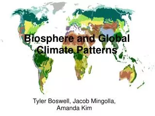
Research Goals Research Goals: • Find global climate patterns of interest to Earth Scientists A key interest is finding connections between the ocean and the land. • Global snapshots of values for a number of variables on land surfaces or water. • Monthly over a range of 10 to 50 years.
Sources of Earth Science Data • Before 1950, very sparse, unreliable data. • Since 1950, reliable global data. • Ocean temperature and pressure are based on data from ships. • Most land data, (solar, precipitation, temperature and pressure) comes from weather stations. • Since 1981, data has been available from earth orbiting satellites. • FPAR, a measure related to plants and greenness • Since 1999 TERRA, the flagship of the NASA earth observing system, is providing much more detailed data.
Importance of Global Climate Patterns • The climate of the Earth’s land surface is strongly influenced by the behavior of the Earth’s oceans. • El Nino is the anomalous warming of the eastern tropical region of the Pacific. • Associated with droughts in Australia and Southern Africa and heavy rainfall along the western coast of South America. El Nino Events Sea Surface Temperature Anomalies off Peru (ANOM 1+2)
Importance of Global Climate Patterns and NPP • Net Primary Production (NPP) is the net assimilation of atmospheric carbon dioxide (CO2) into organic matter by plants. • NPP is driven by solar radiation and can be constrained by precipitation and temperature. • Keeping track of NPP is important because it includes the food source of humans and all other organisms. • Sudden changes in the NPP of a region can have a direct impact on the regional ecology. • NPP is impacted by global climate patterns. • Precipitation and temperature are directly affected by global climate patterns such as El Nino. • Solar radiation is affected indirectly by cloudiness.
Role of Statistics and Data Mining • Previously Earth scientists have relied on statistical techniques. • Hypothesize-and-test paradigm is extremely labor-intensive. • Data mining provides earth scientist with tools that allow them to spend more time choosing and exploring interesting families of hypotheses. • By applying the proposed data mining techniques, some of the steps of hypothesis generation and evaluation will be automated, facilitated and improved. • However, statistics is needed to provide methods for determining the “statistical” significance of results.
Patterns of Interest • Zone Formation • Find regions of the land or ocean which have similar behavior. • Teleconnections • Teleconnections are the simultaneous variation in climate and related processes over widely separated points on the Earth. • Associations • Find relations between climate events and land cover. • River Discharge • Relationship between water discharged from a river and precipitation, climate, and man.
Clustering for Zone Formation • Interested in relationships between regions, not “points.” • For ocean, clustering based on SST (Sea Surface Temperature) or SLP (Sea Level Pressure). • For land, clustering based on NPP or other variables, e.g., precipitation, temperature. • Typically we work with the points. • When “raw” NPP and SST are used, clustering can find seasonal patterns. • Anomalous regions have plant growth patterns which reversed from those typically observed in the hemisphere in which they reside, and are easy to spot.
K-Means Clustering of Raw NPP and Raw SST (Num clusters = 2) Land Cluster Cohesion: North = 0.78, South = 0.59 Ocean Cluster Cohesion: North = 0.77, South = 0.80
Preprocessing • Time series preprocessing issues • Need to remove seasonality • Earth scientists mostly interest in anomalies • Need to remove most of the autocorrelation • Statistical test are affected • Need to remove trends • Normally want to detect patterns and trends separately • Normally interested in similarity once differences in means and scale have been considered. • Pearson’s correlation coefficient has this property
Minneapolis Atlanta Sao Paolo Minneapolis 1.0000 0.7591 -0.7581 Minneapolis Atlanta 0.7591 1.0000 -0.5739 Sao Paolo -0.7581 -0.5739 1.0000 Sample NPP Time Series Correlations between time series
Minneapolis Atlanta Sao Paolo Minneapolis 1.0000 0.0492 0.0906 Minneapolis Atlanta 0.0492 1.0000 -0.0154 Sao Paolo 0.0906 -0.0154 1.0000 Seasonality Accounts for Much Correlation Normalized using monthly Z Score: Subtract off monthly mean and divide by monthly standard deviation Correlations between time series
Preprocessing: Removing Trends A slight linear trend added to two random time series increases their correlation dramatically, from 0.01 to 0.17.
© V. Kumar Discovery of Patterns in the Global Climate System using Data Mining 17 Ocean Climate Indices: Connecting the Ocean and the Land • An OCI is a time series of temperature or pressure • Based on Sea Surface Temperature (SST) or Sea Level Pressure (SLP) • OCIs are important because • They distill climate variability at a regional or global scale into a single time series. • They are well-accepted by Earth scientists. • They are related to well-known climate phenomena such as El Niño.
Ocean Climate Indices – ANOM 1+2 • ANOM 1+2 is associated with El Niño and La Niña. • Defined as the Sea Surface Temperature (SST) anomalies in a regions off the coast of Peru • El Nino is associated with • Droughts in Australia and Southern Africa • Heavy rainfall along the western coast of South America • Milder winters in the Midwest El Nino Events
Connection of ANOM 1+2 to Land Temp OCIs capture teleconnections, i.e., the simultaneous variation in climate and related processes over widely separated points on the Earth.
Ocean Climate Indices - NAO • The North Atlantic Oscillation (NAO) is associated with climate variation in Europe and North America. • Normalized pressure differences between Ponta Delgada, Azores and Stykkisholmur, Iceland. • Associated with warm and wet winters in Europe and in cold and dry winters in northern Canada and Greenland • The eastern US experiences mild and wet winter conditions. Iceland Azores
Influence of OCI on Land – Area Weighted Correlation • Correlation of an OCI with a land variable is a standard way to evaluate its “influence.” • Correlation does not imply causality. • Temperature and precipitation are the typical land variables. • If relatively many land points have a relatively high correlation, then an OCI is influential. • To evaluate whether clusters (or pairs) are potential OCIs we compute their area weighted correlation. • Weighted average of the correlation with land points, where weight is based on area. • May exclude points whose correlation is low and then calculate area weighted correlation.
Evaluation of Known OCIs via Area Weighted Correlation Area Weighted Correlation of Known OCIs to Land Temp Overlapping, threshold = 0
Evaluation of Known OCIs via Area Weighted Correlation … Area weighted correlation declines as we consider only land points whose temperature correlates with the OCI above a given threshold.
Discovering OCIs via Data Mining • Earth scientists have discovered currently known OCIs. • Observation • Eigenvalue techniques such as Principal Components Analysis (PCA) and Singular Value Decomposition (SVD). • Clustering provides an alternative approach. • Clusters represent ocean regions with relatively homogeneous behavior. • The centroids of these clusters are time series that summarize the behavior of these ocean areas, and thus, represent potential OCIs.
Finding Influential Ocean Regions • Not all points on the ocean correlate well with land variables such as temperature and precipitation. • Best points are those which have a high “density” • Dense points are relatively homogenous with respect to their neighboring points.
Discovery of Ocean Climate Indices • Use clustering to find areas of the oceans that have high density, I.e., relatively homogeneous behavior. • Cluster centroids are potential OCIs. • For SLP pairs of cluster centroids are potential OCIs. • Evaluate the “influence” of potential OCIs on land points. • Determine if the potential OCI matches a known OCI. • For potential OCIs that are not well-known, conduct further evaluation. • Are there land points that have higher correlation for the potential OCI than for known indices?
Evaluating Cluster Centroids as Potential OCIs • Evaluation will be based on area weighted correlation • Ignore clusters who area weighted correlation is low. • Three cases: • Clusters are highly similar to known OCIs (corr > 0.4) • May represent a known OCI • Clusters may be “better,” i.e., higher coverage • Clusters may cover different area, i.e., some points for which the new OCI is a better predictor • Clusters are moderately similar to known OCIs ( 0.25 < corr < 0.4 ) • Again, new OCIs may be better predictors for some points. • Clusters are not similar to known OCIs (corr < 0.25) • These clusters may represent as yet undiscovered Earth Science phenomena.
SST Clusters Highly Correlated to Known Indices Area Weighted Correlation of Cluster Centroids to Land Temp Overlapping, threshold = 0
SST Clusters that Correspond to El Nino Climate Indices 75 78 67 94 El Nino Regions Defined by Earth Scientists SNN clusters of SST that are highly correlated with El Nino indices, ~ 0.93 correlation.
SST Clusters Highly Correlated to Known Indices … Examples of some SST clusters that are highly correlated to known OCIs and have high area weighted correlation with land temperature. These indices have a significant correlation with El Nino indices.
SST Clusters Highly Correlated to Known Indices However, there are areas (yellow) where these clusters correlate better.
Comments from our NASA collaborators “Ocean cluster results based on SST correlations with land surface temperature suggest that • New areas of the ocean may be identified that are unknown as being highly representative of the El Nino Southern Oscillation (ENSO) and the Arctic Oscillation (AO).” • New predictive indices for land climate over the past 40 years can be identified that will improve upon predictions using any known ocean climate index to date, including SOI and AO.”
Issues in Mining Associations from Earth Science Data • Data is continuous rather than discrete. • Data has spatial and temporal components. • Data can be multilevel • time and spatial granularities. • Observations are not i.i.d. due to spatial and temporal autocorrelations. • Data may contain noise, missing information and measurement errors • historical SST data between 1856-1941 is measured using wooden buckets. • Data may come from heterogeneous sources • Calibration issues.
Mining Associations in Earth Science Data: Challenges • How to transform Earth Science data into transactions? • What are the “baskets”? • What are the “items”? • How to define “support”?
How to identify interesting patterns? • Use objective interest measures. • Use domain knowledge. Mining Associations Patterns in Earth Science Data: Challenges • How to efficiently discover spatio-temporal associations? • Use existing algorithms. • Develop new algorithms. 1 FPAR-HI PET-HI PREC-HI SOLAR-HI TEMP-HI ==> NPP-HI (support count=145, confidence=100%) 2 FPAR-HI PET-HI PREC-HI TEMP-HI ==> NPP-HI (support count=933, confidence=99.3%) 3 FPAR-HI PET-HI PREC-HI ==> NPP-HI (support count=1655, confidence=98.8%) 4 FPAR-HI PET-HI PREC-HI SOLAR-HI ==> NPP-HI (support count=268, confidence=98.2%) …
Event Definition • Items are events abstracted from time series. • Events of interest include: • Temporal events: • Anomalous temporal events such as warmer winters and droughts. • Changes in the periodic behavior such as longer growing seasons or earlier month of onset of greenup. • Spatial events: • Large percentage of land areas in a certain region having below-average precipitation. • Spatio-temporal events: • Changes in circulation or trajectory of jet-streams.
Example of Anomalous Event Definition If threshold for Z = 1.5, on average, there are ~20 events per time series.
Transaction and Support Definitions • Convert the time series into sequence of events for each spatial location.
Examples of Association Patterns • min support = 0.001%, min confidence=10% 1 FPAR-HI PET-HI PREC-HI SOLAR-HI TEMP-HI ==> NPP-HI (support count=145, confidence=100%) 2 FPAR-HI PET-HI PREC-HI TEMP-HI ==> NPP-HI (support count=933, confidence=99.3%) 3 FPAR-HI PET-HI PREC-HI ==> NPP-HI (support count=1655, confidence=98.8%) 4 FPAR-HI PET-HI PREC-HI SOLAR-HI ==> NPP-HI (support count=268, confidence=98.2%) 5 FPAR-HI PET-HI PREC-HI SOLAR-LO TEMP-HI ==> NPP-HI (support count=44, confidence=97.8%) 6 FPAR-LO PET-LO PREC-LO SOLAR-LO ==> NPP-LO (support count=216, confidence=96.9%) 7 FPAR-LO PREC-LO SOLAR-LO TEMP-HI ==> NPP-LO (support count=152, confidence=96.2%) 8 FPAR-LO PET-LO PREC-LO SOLAR-LO TEMP-LO ==> NPP-LO (support count=47, confidence=95.9%) 9 FPAR-LO PREC-LO SOLAR-LO TEMP-LO ==> NPP-LO (support count=49, confidence=94.2%) 10 FPAR-LO PREC-LO SOLAR-LO ==> NPP-LO (support count=595, confidence=93.7%) … 75 FPAR-HI ==> NPP-HI (support count = 216924, confidence = 55.7%) NPP = Solar * FPAR * * Temperature * Moisture
Shrubland areas Rule has high support in shrubland areas Example of Interesting Association Patterns FPAR-Hi ==> NPP-Hi (sup=5.9%, conf=55.7%)
Land Cover Types Shrublands/
Using Land Cover as Additional Features 1. FPAR-HI PET-HI PREC-HI SOLAR-HI TEMP-HI ==> NPP-HI (support count=145, confidence=100%) 2. FPAR-HI PET-HI PREC-HI SOLAR-HI TEMP-HI GRASSLAND ==> NPP-HI (support count=145, confidence=100%) 3. FPAR-HI PET-HI PREC-HI SOLAR-HI TEMP-HI FOREST ==> NPP-HI (support count=44, confidence=100%) 4. FPAR-HI PET-HI PREC-HI SOLAR-HI TEMP-HI CROPLAND ==> NPP-HI (support count=44, confidence=100%) 5. FPAR-HI PET-HI PREC-HI SOLAR-HI FOREST ==> NPP-HI (support count=75, confidence=100%) 6. FPAR-HI PET-HI PREC-HI SOLAR-HI CROPLAND ==> NPP-HI (support count=81, confidence=100%) 7. FPAR-HI PREC-HI SOLAR-HI TEMP-HI CROPLAND ==> NPP-HI (support count=58, confidence=100%) 8. FPAR-HI PET-HI PREC-HI TEMP-HI GRASSLAND ==> NPP-HI (support count=376, confidence=99.5%) 9. FPAR-HI PET-HI PREC-HI TEMP-HI CROPLAND ==> NPP-HI (support count=170, confidence=99.4%) 10. FPAR-HI PET-HI PREC-HI CROPLAND ==> NPP-HI (support count=277, confidence=99.3%) ….. • Produce multiple rules that have the same form: • {A} ==> {B}, {A,Grassland} ==> B, {A, Cropland} ==> {B}, etc. • Some of the support counts could be missing if itemsets fall below the minimum support threshold.
Finding Interesting Earth-Science Patterns • A pattern is interesting if it occurs relatively more frequently in some homogeneous regions. • If the relative frequency of a pattern is similar in all groups of land areas, then it is less interesting. • If the pattern occurs mostly in a certain group of land areas, then it is potentially interesting.
Filtering Patterns using Land Cover Types • For each pattern p: • Actual coverage for land cover type i = si /S • Expected coverage for land cover type i = ni /N • Ratio of actual to expected coverage for land cover type i, • ei = si N / ni S • Interest Measure • If pattern occurs in arbitrary regions, interest measure will be low.
FPAR-Hi ==> NPP-Hi • FPAR-Hi NPP-Hi tends to occur in shrubland and grassland regions. • Possible explanation: this type of vegetation can take advantage of periodically high precipitation more quickly than forests. • New hypothesis: FPAR-HI events in these regions could be related to unusual precipitation conditions. Forest (0.1%), Croplands (4.2%), Grasslands (25.9%), Desert (3.6%) FPAR-Hi Prec-Hi ==> NPP-Hi Interesting Spatial Association Pattern


![Knowledge Discovery in Data [and Data Mining] (KDD)](https://cdn2.slideserve.com/4256051/knowledge-discovery-in-data-and-data-mining-kdd-dt.jpg)