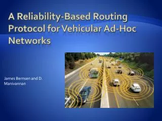
A Reliability-Based Routing Protocol for Vehicular Ad-Hoc Networks

1. James Bernsen and D. Manivannan A Reliability-Based Routing Protocol for Vehicular Ad-Hoc Networks

2. Overview • Introduction • VANETs and their Applications • Routing in a VANET • Related Work • GPSR • GSR, SAR, STAR • RIVER • Reliable Inter-VEhicular Routing

3. Introduction VANETs, Applications, Routing Strategies

4. Vehicular Ad-Hoc Network • A VANET is a wireless network formed between vehicles on an as-needed basis • Special class of mobile ad-hoc networks with some unique characteristics • Nodes generally constrained to roadways • Vehicles move relatively quickly compared to MANETs • Distinct mobility pattern subject to traffic laws • Radio obstacles may be present in urban areas

5. Applications of VANETs • Motor Vehicle Safety • Accident avoidance • Driver alerts • Emergencyvehicle dispatch • Driver Conveniences • Live traffic updates • Find parking spaces • Local shopping and services; points of interest • Traffic signal warnings and optimization • Cooperative driving and Automated driving • Passenger Entertainment

6. VANET Routing • Nodes typically identified by both a network address and a last-known position • Node communication generally short range • Communication over longer distances requires messages to hop through multiple nodes

7. VANET Routing Strategies • Position-based, greedy forwarding • Periodic beacons to determine node neighbors • Some form of street awareness is typical. • Positioning-system (GPS) and a map are commonly required. • GPSR, a MANET protocol, is often used as a starting point. GSR (Other VANET Protocols) GPSR SAR STAR RIVER

8. Related Work MANET and VANET Routing Protocols

9. GPSR • A position-based routing protocol for MANETs • Uses beacons to determine node neighbors. • Greedily forwards messages toward a known destination position • If, at any hop, there are no nodes in the direction of the destination, a recovery mode is used. • This “perimeter mode” converts the node connectivity graph into a planar graph and attempts to route around the network void.

10. GSR • Geographic Source Routing • Uses beacons to determine neighbor node locations • Uses a static street map and routes messages along streets, anchored at intersections. • Recognized weaknesses of GPSR in VANETs • Frequent radio obstacles in urban areas require GPSR to use its perimeter mode frequently. • Lack of greedy forwarding in perimeter mode increases delays and hop counts. • Rapid movement of vehicular nodes can cause loops.

11. SAR • Spatially Aware Routing (SAR) • Uses beacons to determine neighbors • Position-based: sender creates a route to a destination based on immobile physical locations in the street map and stores it in the packet header. • Uses a street map to avoid permanent network voids • Recognized weaknesses of GPSR in VANETs • Permanent network voids (buildings) will repeatedly incur perimeter mode and degrade performance

12. SAR • Suggested these recovery strategies when no node is found along the predetermined route: • Place the packet in a “suspension buffer” • Attempt greedy forwarding, like GPSR • Compute a new route

13. STAR • Spatial and Traffic Aware Routing • Attempts to improve upon SAR by forwarding messages in directions with relatively denser traffic. • Sender provides a partial route to be updated by intermediate nodes along the route. • Uses periodic beacon messages to determine each node’s neighbors and exchange traffic information. • Performs passive traffic monitoring by counting the number of nodes encountered in the cardinal and intercardinal directions relative to each node. • Recognizes temporary and persistent traffic conditions.

14. RIVER Reliable Inter-VEhicular Routing

15. RIVER at a Glance • Position-based; assumes GPS and map • Prefers transmitting messages using routes that it has deemed reliable through traffic monitoring • Real-time traffic monitoring via probe messages and by passive monitoring of other messages • Propagates route reliability information without the use of broadcast or network flooding • Allows dynamic route recalculation and recovery

16. Typical RIVER Network Stack • Depends on 802.11 transmission, MAC protocol, and IP protocol layers beneath. • Provides VANET routing capability to the transport and application layers above.

17. Beaconing • Beacon: a one-hop message sent at a semi-regular interval used to identify neighbor nodes. • Beacon contains: • Beacon sender address (in IP header) • The geolocation of the beacon sender • Timestamp (for freshness of reliability information) • Known reliability of street edges • When a node receives a beacon, it may add/update: • Sender’s information in its neighbors-table • Most recent reliability of street edges in its street graph • Implicit beacons are also sent by piggybacking beacon data on other kinds of RIVER messages.

18. Beaconing • To prevent synchronized sending of beacons, we adjust the frequency with a randomized “jitter” between beacons, as in GPSR. • Neighbors are assumed out-of range and deleted from the neighbor table when: • A preset timeout interval has elapsed without receiving a beacon from that neighbor • The 802.11 MAC layer indicates a link-level transmission failure during the Request-To-Send / Clear-To-Send (RTS/CTS) handshake.

19. RIVER Street Graph • Forms an undirected graph where vertices are intersections or curves in the roadway and edges are the streets that connect those vertices. • Allows routing messages along streets. • G = (V,E) • V = set of vertices • E = set of edges • v ∈ V v = {i, x, y} • i = internal identifier • (x,y) = geolocation • e ∈ E e = {u,v,w} • u, v ∈ V and u ≠ v • w = edge weight

20. RIVER Street Graph • Prevalence of navigation systems make the map requirement a reasonable assumption. • Supports heterogeneous maps by requiring no common naming among nodes for identifying vertices and edges – ID by coordinates only • Coordinates need to be within a reasonable level of accuracy but not exactly the same among nodes: • Node a sends a message containing the coordinates of vertex ua to node b. • Node b will consider uaub if no other vertex in b’s graph has coordinates closer to ua than ub.

21. Traffic Monitoring • Temporary disconnections frequently occur at non-deterministic intervals, partitioning the network. • VANET routing protocols must handle this situation or drop the packet.

22. Active Traffic Monitoring: Probes • A probe message is a RIVER protocol packet that is periodically sent by a node located near a street vertex and forwarded greedily along a street edge that is incident to that vertex. • Sent when the reliability of the edge is unknown or has been untested for a preset interval of time. 

23. Probe Messages • Strictly a protocol message; contains no data payload. • Anycast message: sent to any node in a group of nodes defined by a particular geographic area. The destination node is not known when sent. • If the probe encounters a network gap, it is dropped. • If received, nodes at the receiving vertex become aware that the edge is traversable, and the receiving node sends a return probe.

24. Passive Traffic Monitoring • Every beacon, probe, and routing message contains edge reliability information. • Edges traversed by probe and routing packets • Known Edge List (KEL) – data structure included in all RIVER packets • Weighted Routes – every edge in the path of a routing packet contains a timestamped reliability weight for that edge.

25. Known Edge List (KEL) • List is populated with selected edges from the accumulated reliability information known by the sender of the packet, including: • Reliability rating • Timestamp when the edge reliability was last updated • Edge Sharing Criteria • Edge’s reliability updated since it was last shared • Prefers edges that were updated most recently • Further prefers edges whose reliability is known from first-hand knowledge (not learned from a KEL)

26. Passive Traffic Monitoring • Enables a node to learn about remote edges of the street graph when it receives a message from a distant node. • x – nearby probed edges • y – weighted route path • z – edges contributed to the routing packet’s KEL by forwarding nodes

27. Edge Reliability • To determine a reliable route, a node must be able to choose paths that contain a sufficient density of nodes to maintain communication. • Vehicular nodes move quickly and frequently, so it is infeasible for each node to track all other nodes’ movement across a particular area to determine usable routes. • We hypothesize that it is more efficient to determine if a particular street edge was recently reliable and share this information with others.

28. Determining Reliable Paths • Dijkstra’s algorithm finds the least-weight path • Shortest-path algorithms base edge weights on the physical distance between vertices • RIVER edge weights are an estimate of reliability • Smaller weight  higher reliability, (minimum is zero) • Larger weight  lower reliability, (∞  not traversable)

29. Reliability Calculation • A reliability default value is given to edges with no packet traversal information or where the last known packet traversal was more than reliability default ms ago. • Set to 10,000 ms (10 seconds) • Acts as a timeout value that represents the “reliability unknown” state. • If we don’t have information on an edge in the last 10seconds, then we revert that edge to this “reliability unknown” value. • Untraversable Edge Weight (∞) • Used when a node attempts to forward a packet but can find no neighbor to whom the packet can be sent.

30. Reliability Calculation • First-hand reliability observation: the edge’s reliability = number of milliseconds since the edge was last known to have been traversed by a packet • When a packet is received over edge e, rely(e) = 0 • As time elapses, rely(e) decays to a higher value • Constant multipliers discourage the use of edges that the node considers unreliable. rely(e) = 10000 100000 0 1000 2000 3000 4000 5000 6000 7000 8000 9000 10000

31. RIVER Edge Reliability Traits • Reliable edges have a relatively small range of ratings compared to unreliable edges. • Due to the use of Dijkstra’s algorithm • Intention is to prevent the algorithm from preferring (for example) a single unreliable edge over several reliable edges. • A reliable edge’s rating will time out and return to an “unknown reliability” state. • An unreliable edge’s rating will remain until it is determined to be more reliable. • An unreliable edge rating stabilizes when a node can no longer test the edge by sending probes across it.

32. Routing Source(Sending to node 2) • Select a path based on the reliability of edges in the graph. • Identify the geolocation of the destination node. • If distant, use Dijkstra’s algorithm to calculate the most reliable path to the destination. • Vertices that make up this routing path are anchor points of the route (anchor path). • The path is written to the routing header of the packet. w=8,000 w=10,000 w=10,000 w=10,000 Destination

33. Routing • Node with a packet forwards it along the route in the header. • Consults the routing header for the next anchor point • Refers to its neighbors-table for a node within radio range and closest to the next anchor point • Sets the next-hop address (IP header destination) • Attempts to send the packet • If MAC layer handshake fails, repeat the process Neighbor Next AP

34. Routing • At each hop of the packet, the receiving node: • Checks for destination presence • Performs passive monitoring • Updates its neighbor table with implicit beacon data • Updates its edge weights with KEL and weighted route • Consults the routing header for the next anchor point • If the next anchor point has been reached/passed, advance the pointer until an unreached AP is found • If an anchor point remains, forwarding continues as described. Else, the node forwards greedily toward the destination node. Not Destination Destination not in range Passive Monitor Next AP

35. Route Recovery • If a node can find no next-hop: • Mark the edge untraversable (∞). • Find a new path with Dijkstra’s . • If the new path has a mean weight that is less than the current path’s weight by a significant threshold, overwrite the current path with the new path. • If the new anchor path’s next edge is less than ∞, then the search for a next-hop neighbor resumes recursively. (If no next hop can be found on the new anchor path, the recovery process may be repeated.) • The recovery process is aborted if the anchor path’s next edge is untraversable (∞). The packet is dropped. No Hop to AP! w=∞ Next AP Next AP w=10,000 w=2,000 w=10,000

36. Route Recalculation • Proactive route recovery aimed at preventing a route failure while the packet is at a vertex. • A forwarding node at an anchor point uses Dijkstra’s algorithm to calculate a new proposed route. • If the proposed route has a mean weight that is less than the current path weight by a significant threshold, then the proposed route is used instead. Recalculate w=150,000 w=10,000 12,000 < (160,000 – 5,000) w=2,000 w=10,000

37. Greedy Optimizations • Strict greedy strategy forwards a packet toward the next anchor point until the packet arrives at a node that is within some predefined range of the anchor point, called the vertex range. • Complexities arise due to the differences between the vertex range, each node’s radio range, and the density of traffic. • RIVER has two optimizations to avoid dropping packets unnecessarily. • Past Anchor Point, Outside Zone • Outside Zone, No Closer Neighbor

38. Past Anchor Point, Outside Zone • Current AP: this intersection; next AP is beyond node B. • Node A seeks a node closer to the AP zone than itself, and node B meets the criteria. • However, node B is not within the AP zone, and it will also seek a node closer to the AP (backtracking) when the next AP is in the opposite direction of the current AP! • Since node B is past the current AP along the anchor route, it should plot a path to the next AP instead. A B

39. Outside Zone, No Closer Neighbor • Current AP: this intersection; next AP is beyond node B. • Node A seeks a node closer to the AP zone than itself, but NO node meets the criteria. • However, B is within radio range, and it is located on the edge between this AP and the subsequent AP. • Since node B is past the current AP and closer to the subsequent AP along the anchor route, A should forward to B. A B

40. Performance Evaluation • Simulated the protocol with the ns-2 simulator at version 2.33 using the CMU wireless extension. • Varied parameter settings to test different scenarios and feature sets of RIVER. • RIVER also compared against peer protocols • STAR routing protocol (Giudici, Pagani) • GPSR routing protocol (Karp, Kung) • Short-Path, a generic shortest-path VANET routing algorithm

41. Performance Metrics • Data throughput: mean percentage of routed data packets that were successfully delivered. • Route header size: average size of a routing packet, excluding the data portion. • Forwards per route: average hop count of a data packet to its destination. • Route transit time: number of seconds required to deliver a data packet from its original sender to its final destination.

42. Simulation Parameters • 100-300 vehicular nodes • Velocities: • Min = 11 km/hr • Avg = 36 km/hr • Max = 51 km/hr • 5 sender/receiver pairs selected at random • 200 seconds of simulation • Silent for first 20 seconds and final 16 seconds • 21 transfer attempts between each pair • 8 seconds apart • Different pairs do not transmit simultaneously

43. Route Recalculation and Recovery

44. Route Recalculation and Recovery

45. Route Recalculation and Recovery

46. Route Recalculation and Recovery

47. Reliability Distribution

48. Reliability Distribution

49. Reliability Distribution

50. Probe Messages