Process Dynamics
Refers to unsteady-state or transient behavior. Steady-state vs. unsteady-state behavior Steady state : variables do not change with time But on what scale? cf., noisy measurement ChE curriculum emphasizes steady-state or equilibrium situations: Examples: ChE 10, 110, 120.

Process Dynamics
E N D
Presentation Transcript
Refers to unsteady-state or transient behavior. • Steady-state vs. unsteady-state behavior • Steady state: variables do not change with time • But on what scale? cf., noisy measurement • ChE curriculum emphasizes steady-state or equilibrium situations: • Examples: ChE 10, 110, 120. • Continuous processes: Examples of transient behavior: • Start up & shutdown • Grade changes • Major disturbance: e.g., refinery during stormy or hurricane conditions • Equipment or instrument failure (e.g., pump failure) • Process Dynamics
Batch processes • Inherently unsteady-state operation • Example: Batch reactor • Composition changes with time • Other variables such as temperature could be constant. Process Control • Large scale, continuous processes: • Oil refinery, ethylene plant, pulp mill • Typically, 1000 – 5000 process variables are measured. • Most of these variables are also controlled.
Process Control (cont’d.) • Examples: flow rate, T, P, liquid level, composition • Sampling rates: • Process variables: A few seconds to minutes • Quality variables: once per 8 hr shift, daily, or weekly • Manipulated variables • We implement “process control” by manipulating process variables, usually flow rates. • Examples: feed rate, cooling rate, product flow rate, etc. • Typically, several thousand manipulated variables in a large continuous plant
Process Control (cont’d.) • Batch plants: • Smaller plants in most industries • Exception: microelectronics (200 – 300 processing steps). • But still large numbers of measured variables. • Question: How do we control processes? • We will consider an illustrative example.
1.1 Illustrative Example: Blending system • Notation: • w1, w2 and w are mass flow rates • x1, x2 and x are mass fractions of component A
Assumptions: • w1 is constant • x2 = constant = 1 (stream 2 is pure A) • Perfect mixing in the tank Control Objective: Keep x at a desired value (or “set point”) xsp, despite variations in x1(t). Flow rate w2 can be adjusted for this purpose. • Terminology: • Controlled variable (or “output variable”): x • Manipulated variable (or “input variable”): w2 • Disturbance variable (or “load variable”): x1
Design Question. What value of is required to have Overall balance: Component A balance: (The overbars denote nominal steady-state design values.) • At the design conditions, . Substitute Eq. 1-2, and , then solve Eq. 1-2 for :
Equation 1-3 is the design equation for the blending system. • If our assumptions are correct, then this value of will keep at . But what if conditions change? Control Question. Suppose that the inlet concentration x1 changes with time. How can we ensure that x remains at or near the set point ? As a specific example, if and , then x > xSP. • Some Possible Control Strategies: • Method 1. Measure x and adjust w2. • Intuitively, if x is too high, we should reduce w2;
Manual control vs. automatic control • Proportional feedback control law, • where Kc is called the controller gain. • w2(t) and x(t) denote variables that change with time t. • The change in the flow rate, is proportional to the deviation from the set point, xSP – x(t).
Method 2. Measure x1 and adjust w2. • Thus, if x1 is greater than , we would decrease w2 so that • One approach: Consider Eq. (1-3) and replace and with x1(t) and w2(t) to get a control law:
Because Eq. (1-3) applies only at steady state, it is not clear how effective the control law in (1-5) will be for transient conditions. • Method 3.Measure x1 and x, adjust w2. • This approach is a combination of Methods 1 and 2. • Method 4. Use a larger tank. • If a larger tank is used, fluctuations in x1 will tend to be damped out due to the larger capacitance of the tank contents. • However, a larger tank means an increased capital cost.
1.2 Classification of Control Strategies Table. 1.1 Control Strategies for the Blending System • Feedback Control: • Distinguishing feature: measure the controlled variable
It is important to make a distinction between negative feedback and positive feedback. • Engineering Usage vs. Social Sciences • Advantages: • Corrective action is taken regardless of the source of the disturbance. • Reduces sensitivity of the controlled variable to disturbances and changes in the process (shown later). • Disadvantages: • No corrective action occurs until after the disturbance has upset the process, that is, until after x differs from xsp. • Very oscillatory responses, or even instability…
Feedforward Control: • Distinguishing feature: measure a disturbance variable • Advantage: • Correct for disturbance before it upsets the process. • Disadvantage: • Must be able to measure the disturbance. • No corrective action for unmeasured disturbances.