Download
1 / 65
650 likes | 848 Vues
Results from the Telescope Array Experiment. Gordon Thomson University of Utah. Outline. Introduction TA Results: Spectrum Composition Search for anisotropy Search for photon, neutrino events Future projects: TALE, Radar Conclusions. Cosmic Rays Cover a Wide Energy Range.

E N D
Results from the Telescope Array Experiment Gordon Thomson University of Utah LBL, April 10, 2012
Outline • Introduction • TA Results: • Spectrum • Composition • Search for anisotropy • Search for photon, neutrino events • Future projects: TALE, Radar • Conclusions
Cosmic Rays Cover a Wide Energy Range At lower energies, spectrum of cosmic rays is almost featureless. Only the “knee” at 3x10¹⁵ eV The knee is due to a rigidity-dependent cutoff, seen in composition. Kascade experiment: measures electron and muon components of showers. Model dependent, but indicative. Is it Emax or containment? Low energy (Ec=3x10¹⁷ eV) and sharp elemental cutoffs limit comes from Emax, rather than containment. Learn about galactic sources. Structure Physics
Cosmic Rays Cover a Wide Energy Range At lower energies, spectrum of cosmic rays is almost featureless. Only the “knee” at 3x10¹⁵ eV The knee is due to a rigidity-dependent cutoff, seen in composition. Kascade experiment: measures electron and muon components of showers. Model dependent, but indicative. Is it Emax or containment? Low energy (Ec=3x10¹⁷ eV) and sharp elemental cutoffs limit comes from Emax, rather than containment. Learn about galactic sources. Structure Physics p Fe
Has the Fe knee been seen? • Kascade-Grande Experiment, 2011, measuring electron and muon intensities, may be seeing the Fe end of the Emax transition. All-particle spectrum Muon-rich events (high z)
Big Change Expected at High Energies Expect two spectral features due to interactions between CR protons and CMBR photons. GZK cutoff due to pion production. Dip in spectrum due to e+e- pair production (the ankle). Galactic/extragalactic transition. Galactic (supernova remnants) give heavy composition, extragalactic (AGN’s) give light composition. A third spectral feature is seen, second knee. Learn about extragalactic sources; and propagation over cosmic distances.
A Second Rigidity-Dependent Cycle? • Galactic magnetic field: • Regular component ~3μG, follows the spiral arms • Random component ~5μG, 50-100 pc coherence length • Critical energy, where Larmor radius = coherence length: Ec ~ 1017.5 eV for protons, 1018.9 eV for Fe • Confinement for galactic particles; • Exclusion for extragalactic particles • Galactic – extragalactic transition. Emax Ec
A Second Rigidity-dependent Cycle? • HiRes prototype+MIA hybrid experiment, 1999. • Best evidence for galactic-extragalactic transition
Today’s Issues • Anisotropy. What are the sources? • The biggest question. • Both galactic and extragalactic magnetic fields get in the way: the highest energy events are important. • Composition. Protons, Fe, or what? • How does composition vary with energy? • Disagreement among experiments. • Spectrum. • There exists an absolute energy calibration: the GZK cutoff 5-6x10¹⁹ eV --- if protons. GZK develops in ~50 Mpc. • If heavy nuclei, spallation breaks them up above ~4x10¹⁹ eV, and distances < 50 Mpc. • Everything talks to composition.
Cast of Characters • Telescope Array (TA) Experiment • Located in Utah. • Largest experiment in northern hemisphere. • High Resolution Fly’s Eye (HiRes) Experiment • Located in Utah. • Pierre Auger (PAO) Observatory • Located in Argentina. • Largest experiment. • Akeno Giant Air Shower Array (AGASA) • Kascade, Kascade-Grande
Telescope Array Collaboration T Abu-Zayyad1, R Aida2, M Allen1, R Azuma3, E Barcikowski1, JW Belz1, T Benno4, DR Bergman1, SA Blake1, O Brusova1, R Cady1, BG Cheon6, J Chiba7, M Chikawa4, EJ Cho6, LS Cho8, WR Cho8, F Cohen9, K Doura4, C Ebeling1, H Fujii10, T Fujii11, T Fukuda3, M Fukushima9,22, D Gorbunov12, W Hanlon1, K Hayashi3, Y Hayashi11, N Hayashida9, K Hibino13, K Hiyama9, K Honda2, G Hughes5, T Iguchi3, D Ikeda9, K Ikuta2, SJJ Innemee5, N Inoue14, T Ishii2, R Ishimori3, D Ivanov5, S Iwamoto2, CCH Jui1, K Kadota15, F Kakimoto3, O Kalashev12, T Kanbe2, H Kang16, K Kasahara17, H Kawai18, S Kawakami11, S Kawana14, E Kido9, BG Kim19, HB Kim6, JH Kim6, JH Kim20, A Kitsugi9, K Kobayashi7, H Koers21, Y Kondo9, V Kuzmin12, YJ Kwon8, JH Lim16, SI Lim19, S Machida3, K Martens22, J Martineau1, T Matsuda10, T Matsuyama11, JN Matthews1, M Minamino11, K Miyata7, H Miyauchi11, Y Murano3, T Nakamura23, SW Nam19, T Nonaka9, S Ogio11, M Ohnishi9, H Ohoka9, T Okuda11, A Oshima11, S Ozawa17, IH Park19, D Rodriguez1, SY Roh20, G Rubtsov12, D Ryu20, H Sagawa9, N Sakurai9, LM Scott5, PD Shah1, T Shibata9, H Shimodaira9, BK Shin6, JD Smith1, P Sokolsky1, TJ Sonley1, RW Springer1, BT Stokes5, SR Stratton5, S Suzuki10, Y Takahashi9, M Takeda9, A Taketa9, M Takita9, Y Tameda3, H Tanaka11, K Tanaka24, M Tanaka10, JR Thomas1, SB Thomas1, GB Thomson1, P Tinyakov12,21, I Tkachev12, H Tokuno9, T Tomida2, R Torii9, S Troitsky12, Y Tsunesada3, Y Tsuyuguchi2, Y Uchihori25, S Udo13, H Ukai2, B Van Klaveren1, Y Wada14, M Wood1, T Yamakawa9, Y Yamakawa9, H Yamaoka10, J Yang19, S Yoshida18, H Yoshii26, Z Zundel1 1University of Utah, 2University of Yamanashi, 3Tokyo Institute of Technology, 4Kinki University, 5Rutgers University, 6Hanyang University, 7Tokyo University of Science, 8Yonsei University, 9Institute for Cosmic Ray Research, University of Tokyo, 10Institute of Particle and Nuclear Studies, KEK, 11Osaka City University, 12Institute for Nuclear Research of the Russian Academy of Sciences, 13Kanagawa University, 14Saitama University, 15Tokyo City University, 16Pusan National University, 17Waseda University, 18Chiba University 19Ewha Womans University, 20Chungnam National University, 21University Libre de Bruxelles, 22University of Tokyo, 23Kochi University, 24Hiroshima City University, 25National Institute of Radiological Science, Japan, 26Ehime University U.S., Japan, Korea, Russia, Belgium
TA is a Hybrid Experiment • TA is in Millard Co., Utah, 2 hours drive from SLC. • SD: 507 scintillation counters, 1.2 km spacing, scintillator area= 3 sq. m., two layers. • FD: 3 sites, each covers 120° az., 3°-31° elev. • ~3.8 years of data have been collected.
TA Fluorescence Detectors Refurbished from HiRes Middle Drum 14 cameras/station 256 PMTs/camera Observation started Dec. 2007 5.2 m2 ~30km New FDs 256 PMTs/camera HAMAMATSU R9508 FOV~15x18deg 12 cameras/station Observation started Nov. 2007 Black Rock Mesa Long Ridge Observation started Jun. 2007 13 6.8 m2 ~1 m2
Typical Fluorescence Event Black Rock Event Display Fluorescence Direct (Cerenkov) Rayleigh scatt. Aerosol scatt. Monocular timing fit Reconstructed Shower Profile
TA Surface Detector • Powered by solar cells; radio readout. • Self-calibration using single muons. • In operation since March, 2008.
r = 800m Typical surface detector event 2008/Jun/25 - 19:45:52.588670 UTC Geometry Fit (modified Linsley) Fit with AGASA LDF • S(800): Primary Energy • Zenith attenuation by MC • (not by CIC). Lateral Density Distribution Fit
Stereo and Hybrid Observation • Many events are seen by several detectors. • FD mono has ~5° angular resolution. • Add SD information (hybrid reconstruction) ~0.5° resolution. • Stereo FD resolution ~0.5° • Need stereo or hybrid for composition analysis. • Independent operation until 2010. • Hybrid trigger is in operation now.
Cosmic Ray Spectrum • Status: the GZK cutoff was first observed by HiRes; Auger sees it also. • The ankle shows up clearly in both spectra.
TA Spectrum (Measured by the Surface Detector) • 3 years of data, 10997 events. • We use a new analysis method. • Must cut out SD events with bad resolution. Must calculate aperture by Monte Carlo technique. • This is an important part of UHECR technique, and must be done accurately. • We use HEP methods for this purpose.
SD Monte Carlo • Simulate the data exactly as it exists. • Start with previously measured spectrum and composition. • Use Corsika/QGSJet events (solve “thinning” problem). • Throw with isotropic distribution. • Simulate trigger, front-end electronics, DAQ. • Write out the MC events in same format as data. • Analyze the MC with the same programs used for data. • Test with data/MC comparison plots.
How to Use Corsika Events 10-6 thinning • Use 10-6 – thinned CORSIKA QGSJET-II proton showers that are de-thinned in order to restore information in the tail of the shower. • De-thinning procedure is validated by comparing results with un-thinned CORSIKA showers, obtained by running CORSIKA in parallel • We fully simulate the SD response, including actual FADC traces RMS Thinned No thinning Mean VEM / Counter De-thinned De-thinned No thinning Distance from Core, [km]
Dethinning Technique • Change each Corsika “output particle” of weight w to w particles; distribute in space and time. • Time distribution agrees with unthinned Corsika showers.
Fitting results DATA • Fitting procedures are derived solely from the data Time fit residual over sigma Counter signal, [VEM/m2]
Fitting results DATA • Fitting procedures are derived solely from the data • Same analysis is applied to MC • Fit results are compared between data and MC • MC fits the same way as the data. • Consistency for both time fits and LDF fits. • Corsika/QGSJet-II and data have same lateral distributions! Time fit residual over sigma MC Counter signal, [VEM/m2]
Data/MC Comparisons Zenith angle Azimuth angle
Data/MC Comparisons Core Position (E-W) Core Position (N-S)
Data/MC Comparisons LDF χ2/dof Counter pulse height
Data/MC Comparisons S800 Energy
First Estimate of Energy • Energy table is constructed from the MC • First estimation of the event energy is done by interpolating between S800 vs sec(θ) lines
Energy Scale • SD and FD energy estimations disagree • FD estimate possesses less model-dependence • Set SD energy scale to FD energy scale using well-reconstructed events from all 3 FD detectors • 27% renormalization.
SD Energy Spectrum:Broken Power Law Fit GZK: pion photoproduction Ankle: e+e- production
SD Energy Spectrum:Integral Flux E1/2 Measurement E1/2 = 1019.69 eV Berezinsky et al. predict 1019.72 eV
Comparison with theoretical model • Assume constant density of sources, calculate the “modification factor” due to propagation; compare with HiRes and TA data.
SD Energy Spectrum:Comparison ● TA SD ▲ HiRes-I ▼ HiRes-II
SD Energy Spectrum:Comparison ● TA SD ■ Auger 2008 (PRL) +20% ▲ Auger 2011 (ICRC) +20%
Fluorescence Detector (FD) Monocular Spectrum • For FD (mono, hybrid, stereo) measurements, the aperture depends significantly on energy. Must calculate it by Monte Carlo technique. • This is an important part of UHECR technique, and must be done accurately. • We use HEP methods for this purpose.
MC Method • Simulate the data exactly as it exists. • Start with previously measured spectrum and composition. • Use Corsika/QGSJet events. • Throw with isotropic distribution. • Include atmospheric scattering. • Simulate trigger, front-end electronics, DAQ. • Write out the MC events in same format as data. • Analyze the MC with the same programs used for data. • Test with data/MC comparison plots. • This method works.
DATA/MC Comparisons Rp Zenith angle
Composition from Xmax • Shower longitudinal development depends on primary particle type. • FD observes shower development directly. • Xmax is the most efficient parameter for determining primary particle type. HiRes PRL.104.161101 (2010) Shower longitudinal development Number of charged particle Xmax Auger PRL.104.091101 (2010) Depth [g/cm2]
TA FD Stereo Composition • Measure xmax for Black Rock/Long Ridge FD stereo events • Create simulated event set • Apply exactly the same procedure as with the data • This measurement is independent of HiRes and Auger.
Data/MC Comparison QGSJETII Proton Iron Zenith Azimuth Rp Xcore Ycore Psi
Data/MC Comparison QGSJETII Proton Iron Track length # of P.E. # of PMT Likelihood Xstart Xend
Prediction of <Xmax>, Reconstructed These rails which include acceptance and reconstruction bias can be compared with data
Xmax distribution (1018-20eV) Proton Iron QGSJET01 SIBYLL QGSJET-II Preliminary Preliminary Preliminary
Xmax dist. QGSJET-II 18.2 < logE < 18.4 18.4 < logE < 18.6 Preliminary Preliminary 18.6 < logE < 18.8 18.8 < logE < 19.0 Preliminary Preliminary