Download
1 / 32
320 likes | 716 Vues
An Optimal Nearly-Analytic Discrete Method for 2D Acoustic and Elastic Wave Equations. Dinghui Yang Depart. of Math., Tsinghua University Joint with Dr. Peng, McMaster University Supported by the MCME of China and the MITACS. Outline. Introduction

E N D
An Optimal Nearly-Analytic Discrete Method for 2D Acoustic and Elastic Wave Equations Dinghui Yang Depart. of Math., Tsinghua University Joint with Dr. Peng, McMaster University Supported by the MCME of China and the MITACS
Outline • Introduction • Basic Nearly-Analytic Discrete Method(NADM) • Optimal Nearly-Analytic Discrete Method (ONADM) • Numerical Errors and Comparisons • Wave-Field Modeling • Conclusions
Introduction Computational Geophysics Geophysics: a subject of studying the earth problems such as inner structure and substance, earthquake, motional and changing law, and evolution process of the earth. Computational Geophysics: a branch of Geophysics, using computational mathematics to study Geophysical problems. Example: Wave propagation.
Model • Problems to be solved: acoustic and elastic wave equations derived from Geophysics. • Computational Issues: • numerical dispersion, computational efficiency, computational costs and storages, accuracy.
Mathematical Model For the 2D case, the wave equation can be written as (1) displacement component, Stress, Force source. Let
Computational Methods • High-order finite-difference (FD) schemes (Kelly et al.,1976; Wang et al., 2002) • Lax-Wendroff methods (Dablain, 86) • Others like optimally accurate schemes (Geller et al., 1998, 2000), pseudo-spectral methods (Kosloff et al., 1982)
Basic Nearly-Analytic Discrete Method (NADM) Using the Taylor expansion, we have (2) (3) Where denotes the time increment. We converted these high-order time derivatives to the spatial derivatives and included in Eqs. (2) and (3).
Actually, equation (1) can be rewritten as follows with the operators Where and are known elastic constant matrices. So we have
etc. To determine the high-order spatial derivatives, the NADM introduced the following interpolation function
Interpolation connections At the grid point (i-1, j):
Spatial derivatives expressed in term of the wave displacement and its gradients. etc.
Ideas: use the forward FD to approximate the derivatives of the so-called “velocity” , i.e., Computational Cost and Accuracy: • Needs to compute the so-called velocity and it’s derivatives. • In total, 57 arrays are needed for storing the displacement U, the velocity, and their derivatives. • 2-order accuracy in time (Yang, et al 03)
Optimal Nearly-Analytic Discrete Method Improving NADM: • Reduce additional computational cost • Save storage in computation • Increase time accuracy Observation We have
Merits ofONADM • No needs to compute the velocity and it’s derivatives in (4); • Save storage (53%): in total only 27 arrays are used based on the formula (6); • Higher time accuracy: ONADM (4-order) VS NADM(2-order); • ONADM enjoys the same space accuracy as NADM.
Numerical Errors and comparisons The relative errors are defined by for the 1D case and for the 2D case
1D case Initial problem and Its exact solution
Fig. 1. The relative errors of the Lax-Wendroff correction (line 1), the NADM (line 2), and the ONADM (line 3).
Fig. 2. The relative errors of the Lax-Wendroff correction (line 1), the NADM (line 2), and the ONADM (line 3).
2D case Initial problem Its exact solution
Fig. 3. The relative errors of the second-order FD (line 1), the NADM (line 2), and the ONADM (line 3) for case 1.
Fig. 4. The relative errors of the second-order FD (line 1), the NADM (line 2), and the ONADM (line 3) for case 2.
Fig. 5. The relative errors of the second-order FD (line 1), the NADM (line 2), and the ONADM (line 3) for case 3.
Wave field modeling Wave propagation equations The time variation of the source function fi is with f0=15 Hz.
Fig. 6. Three-component snapshots at time 1.4s, computed by the NADM. Fig. 7. Three-component snapshots at time 1.4s, computed by the ONADM. It took about 3.4 minutes.
Conclusions • The new ONADM is proposed. • The ONADM is more accurate than the NADM, Lax-Wendroff, and second-order methods. • Significant improvement over NADM in storage (53%) and computational cost (32%). • Much less numerical dispersion confirmed by numerical simulation.
Future works • Theoretical analyses in numerical dispersion, stability, etc. • Applications in heterogeneous and porous media cases. • 3-D ONADM.